Introduction

This section describes how confidence intervals were estimated, as well as presenting numeric tables of characteristics of all variables involved.

source("baseline-datasetup.R")

# summarytools::view(summarytools::dfSummary(df), file = "./codebook_concise.html")

Means with CIs taking clustering into account

The code chunks create linear models for all variables. The results are used to estimate confidence intervals and intra-class correlations (ICC).

The CIs are calculated with a multilevel model, accounting for school and classroom membership.

# Create a vector with all names of the variables we want. Exclude T3 variables.
names <- df %>% dplyr::select(-id, -intervention, -group, -school, -girl, -SB_selfRepSitbreaksDidNotSit30min_T1, -track, -trackSchool, -contains("_T3"), -contains("_diff")) %>% names(.)

# Create empty soon-to-be-filled objects
m <- NA
mean <- NA
m_p <- NA
ci_low <- NA
ci_high <- NA
ICC_group <- NA
ICC_School <- NA
nonmissings <- NA

## # Use this to test a single variable:
## dftest <- df #%>% na.omit()
## m <- lme4::lmer(mvpaAccelerometer_T1 ~ (1|school) + (1|group), data=dftest)
## mean <- lme4::fixef(m)
## m_p <- profile(m, which = "beta_")
## ci_low <- confint(m_p)[, 1]
## ci_high <- confint(m_p)[, 2]
## ICC_group <- sjstats::icc(m)[1]
## ICC_School <- sjstats::icc(m)[2]
## nonmissings <- length(m@resp$y)


# # UNCOMMENT below and run code

# for (i in names){ # Loop over each variable name for all participants, extract statistics
# m <- lme4::lmer(paste0(i," ~ (1|school) + (1|group)"), data=df)
# mean[i] <- lme4::fixef(m)
# m_p <- profile(m, which = "beta_")
# ci_low[i] <- confint(m_p)[, 1]
# ci_high[i] <- confint(m_p)[, 2]
# ICC_group[i] <- sjstats::icc(m)[1]
# ICC_School[i] <- sjstats::icc(m)[2]
# nonmissings[i] <- length(m@resp$y)
# }
#
# vardatatable <- data_frame(
#   Variable = stringr::str_sub(names(mean), end = -4), #remove "_T1" from names
#   "Mean" = round(mean, 1) %>% format(., nsmall = 1),
#   "CI95" = paste(round(ci_low, 1) %>% format(., nsmall = 1), " - ", round(ci_high, 1) %>% format(., nsmall = 1)),
#   "ICC class" =ifelse(round(ICC_group, 3) == 0, "< 0.001", round(ICC_group, 3) %>% format(., nsmall = 3)),
#   "ICC school" = ifelse(round(ICC_School, 3) == 0, "< 0.001", round(ICC_School, 3) %>% format(., nsmall = 3)),
#   n = nonmissings) %>%
#   dplyr::arrange(Variable) %>%
#   dplyr::filter(Variable != "") %>% #remove first row, which is empty
#   as.data.frame()
#
# ci_total <- data_frame(
#   "ciLo" = ci_low,
#   "mean" = mean,
#   "ciHi" = ci_high,
#   "diamondlabels" = names(mean)) %>%
#   dplyr::filter(diamondlabels != "") %>% #remove first row, which is empty
#   as.data.frame()
#
# # To improve readability, change the variables which are expressed in minutes, to the form "Xh Ymin"
# timeVariables <- c("mvpaAccelerometer", "mpaAccelerometer", "vpaAccelerometer", "lpaAccelerometer", "weartimeAccelerometer", "sitLieAccelerometer", "standingAccelerometer", "mvpaAccelerometer_noCutOff", "mpaAccelerometer_noCutOff", "vpaAccelerometer_noCutOff", "lpaAccelerometer_noCutOff", "weartimeAccelerometer_noCutOff", "sitLieAccelerometer_noCutOff", "standingAccelerometer_noCutOff")
#
# for (variableToChange in timeVariables) {
# originalMean <- vardatatable[vardatatable$Variable == variableToChange, "Mean"] %>% as.numeric()
# newMean <- paste0(floor(originalMean/60), "h ", round(originalMean, 0) %% 60, "min")
# vardatatable[vardatatable$Variable == variableToChange, "Mean"] <- newMean
# originalCI <- vardatatable[vardatatable$Variable == variableToChange, "CI95"]
# originalCIL <- stringi::stri_extract_first_words(originalCI) %>% as.numeric()
# originalCIH <- stringi::stri_extract_last_words(originalCI) %>% as.numeric()
# newCI <- paste0(floor(originalCIL/60), "h ", round(originalCIL, 0) %% 60, "min - ",
#                 floor(originalCIH/60), "h ", round(originalCIH, 0) %% 60, "min")
# vardatatable[vardatatable$Variable == variableToChange, "CI95"] <- newCI
# }
#
# save(vardatatable, file = "./Rdata_files/vardatatable.Rdata")
# save(ci_total, file = "./Rdata_files/ci_total.Rdata")
load("./Rdata_files/vardatatable.Rdata")
load("./Rdata_files/ci_total.Rdata")


vardatatable2 <- vardatatable
vardatatable2$Variable <- gsub("mvpaAccelerometer", "Daily moderate-to-vigorous PA time (accelerometer)*", vardatatable2$Variable)
vardatatable2$Variable <- gsub("padaysLastweek", "Number of days with >30 MVPA min previous week (self-report)*", vardatatable2$Variable)
vardatatable2$Variable <- gsub("sitLieAccelerometer", "Daily time spent sitting or lying down (accelerometer)*", vardatatable2$Variable)
vardatatable2$Variable <- gsub("sitBreaksAccelerometer", "Daily number of times sitting was interrupted (accelerometer)*", vardatatable2$Variable)
vardatatable2$Variable <- gsub("lpaAccelerometer", "Daily light PA time (accelerometer)", vardatatable2$Variable)
vardatatable2$Variable <- gsub("standingAccelerometer", "Daily standing time (accelerometer)", vardatatable2$Variable)

vardatatable2 <- vardatatable2 %>% 
  dplyr::filter(Variable == "Daily moderate-to-vigorous PA time (accelerometer)*" | 
           Variable == "Daily time spent sitting or lying down (accelerometer)*" |
           Variable == "Daily number of times sitting was interrupted (accelerometer)*" |
           Variable == "Number of days with >30 MVPA min previous week (self-report)*" |
           Variable == "Daily light PA time (accelerometer)" |
           Variable == "Daily standing time (accelerometer)") %>% 
  dplyr::mutate(orderVariable = ifelse(`Variable` == "Daily moderate-to-vigorous PA time (accelerometer)*", "a",
                                ifelse(`Variable` == "Daily light PA time (accelerometer)", "b",
                                ifelse(`Variable` == "Daily standing time (accelerometer)", "c",
                                ifelse(`Variable` == "Daily time spent sitting or lying down (accelerometer)*", "d",
                                ifelse(`Variable` == "Daily number of times sitting was interrupted (accelerometer)*", "e",
                                ifelse(`Variable` == "Number of days with >30 MVPA min previous week (self-report)*", "f", NA))))))) %>% 
  dplyr::arrange(orderVariable) %>% 
  dplyr::select(-orderVariable)

vardatatable2 %>% 
    papaja::apa_table(
        caption = "Primary outcome variables with their class and school ICCs. Primary outcome variables highlighted with asterisks.",
        escape = TRUE, format.args = list(digits = c(3, 0), margin = 2)
        )

(#tab:primary-outcome-vars-table-total) Primary outcome variables with their class and school ICCs. Primary outcome variables highlighted with asterisks.

Variable	Mean	CI95	ICC class	ICC school	n
Daily moderate-to-vigorous PA time (accelerometer)*	1h 5min	0h 57min - 1h 13min	0.089	0.062	731
Daily light PA time (accelerometer)	2h 51min	2h 32min - 3h 9min	0.111	0.110	731
Daily standing time (accelerometer)	1h 24min	1h 15min - 1h 34min	0.122	0.041	731
Daily time spent sitting or lying down (accelerometer)*	8h 44min	8h 4min - 9h 24min	0.115	0.138	731
Daily number of times sitting was interrupted (accelerometer)*	25.8	23.5 - 28.0	0.047	0.080	731
Number of days with >30 MVPA min previous week (self-report)*	2.8	2.6 - 3.0	0.047	< 0.001	1082

All main variables, their means, CIs and ICCs.

Values calculated with a multilevel model accounting for school and classroom.


vardatatable %>%
   DT::datatable( #papaja::apa_table(
        caption = "All variables with their class and school ICCs (values calculated with a multilevel model accounting for school and classroom)",
        escape = TRUE #, format.args = list(digits = c(1, 3, 0), margin = 2)
   )

Assorted tables with ICCs

Description

See tabs above for differently sorted tables

Model with school and class: ICC top 20 items, sorted by classroom ICC


vardatatable %>% 
  dplyr::select(Variable, `ICC class`, `ICC school`, n) %>% 
  arrange(desc(`ICC class`)) %>% slice(1:20) %>% 
  as.tbl() %>% 
  papaja::apa_table(caption = "Intra-class correlations sorted by classroom ICC",
        format.args = list(digits = c(3, 0), margin = 2))

(#tab:icc-school-class-sortbyclass) Intra-class correlations sorted by classroom ICC

Variable	ICC class	ICC school	n
standingAccelerometer	0.122	0.041	731
sitLieAccelerometer	0.115	0.138	731
PA_intention_02	0.112	< 0.001	1073
lpaAccelerometer	0.111	0.110	731
sitLieAccelerometer_noCutOff	0.109	0.128	895
standingAccelerometer_noCutOff	0.109	0.045	895
PA_intention	0.106	< 0.001	1073
lpaAccelerometer_noCutOff	0.096	0.098	895
pafreqUsually	0.095	0.002	1082
mpaAccelerometer	0.092	0.087	731
mvpaAccelerometer	0.089	0.062	731
PA_intention_01	0.089	< 0.001	1073
pahrsUsually	0.085	0.004	1082
SB_selfRepSitbreaksWorkPlacement	0.082	0.028	1020
mpaAccelerometer_noCutOff	0.078	0.090	895
mvpaAccelerometer_noCutOff	0.077	0.065	895
walkStepsAccelerometer	0.075	0.074	731
PA_intrinsic	0.074	< 0.001	1074
PA_autonomous	0.073	< 0.001	1078
PA_autonomous_07	0.073	0.005	1070

Model with school and class: ICC top 20 items, sorted by school ICC


vardatatable %>% dplyr::select(Variable, `ICC class`, `ICC school`, n) %>% 
  arrange(desc(`ICC school`)) %>% 
  slice(1:20) %>% 
  papaja::apa_table(caption = "Intra-class correlations sorted by school ICC",
        format.args = list(digits = c(3, 0), margin = 2))

(#tab:icc-school-class-sortbyschool) Intra-class correlations sorted by school ICC

Variable	ICC class	ICC school	n
sitLieAccelerometer	0.115	0.138	731
sitLieAccelerometer_noCutOff	0.109	0.128	895
fatpct	0.002	0.123	942
lpaAccelerometer	0.111	0.110	731
lpaAccelerometer_noCutOff	0.096	0.098	895
mpaAccelerometer_noCutOff	0.078	0.090	895
mpaAccelerometer	0.092	0.087	731
sitBreaksAccelerometer	0.047	0.080	731
walkStepsAccelerometer_noCutOff	0.067	0.077	895
walkStepsAccelerometer	0.075	0.074	731
mvpaAccelerometer_noCutOff	0.077	0.065	895
mvpaAccelerometer	0.089	0.062	731
SB_avgDailySelfRepSittingHoursLastWeekWeekend	0.046	0.055	1062
SB_avgDailySelfRepSittingHoursLastWeekWeekday	0.037	0.054	1062
weartimeAccelerometer	0.028	0.046	731
standingAccelerometer_noCutOff	0.109	0.045	895
standingAccelerometer	0.122	0.041	731
symptom	0.023	0.039	1084
sitBreaksAccelerometer_noCutOff	0.044	0.037	895
SB_intention	0.014	0.035	1064

Model with school, class and educational track

The model below is the same as the one above, except it adds educational track.

#library(sjstats)
#library(lme4)

names <- df %>% dplyr::select(-id, -intervention, -group, -school, -girl, -SB_selfRepSitbreaksDidNotSit30min_T1, -track, -trackSchool, -contains("_T3"), -contains("_diff")) %>% names(.)

# Create empty soon-to-be-filled objects
m <- NA
mean <- NA
m_p <- NA
ci_low <- NA
ci_high <- NA
ICC_group <- NA
ICC_School <- NA
nonmissings <- NA
ICC_track <- NA


## To test the code with a single variable:
# dftest <- df #%>% na.omit()
# m <- lme4::lmer(sitLieAccelerometer_T1 ~ (1|school) + (1|group) + (1|track), data=df)
# mean <- lme4::fixef(m)
# m_p <- profile(m)
# ci_low <- confint(m_p)[5]
# ci_high <- confint(m_p)[10]
# ICC_group <- icc(m)[1]
# ICC_School <- icc(m)[2]
# nonmissings <- length(m@resp$y)

# # UNCOMMENT below and run code

# for (i in names){ # Loop over each variable name for all participants, extract statistics
# m <- lme4::lmer(paste0(i," ~ (1|school) + (1|group) + (1|track)"), data=df)
# mean[i] <- lme4::fixef(m)
# m_p <- profile(m, which = "beta_")
# ci_low[i] <- confint(m_p)[1]
# ci_high[i] <- confint(m_p)[2]
# ICC_group[i] <- sjstats::icc(m)[1]
# ICC_School[i] <- sjstats::icc(m)[3]
# ICC_track[i] <- sjstats::icc(m)[2]
# nonmissings[i] <- length(m@resp$y)
# }
# 
# vardatatable_containing_edutrack <- data_frame(
#   Variable = stringr::str_sub(names(mean), end = -4), #remove "_T1" from names
#   "Mean" = round(mean, 1) %>% format(., nsmall = 1),
#   "CI95" = paste(round(ci_low, 1) %>% format(., nsmall = 1), " - ", round(ci_high, 1) %>% format(., nsmall = 1)),
#   "ICC class" =ifelse(round(ICC_group, 3) == 0, "< 0.001", round(ICC_group, 3) %>% format(., nsmall = 3)),
#   "ICC school" = ifelse(round(ICC_School, 3) == 0, "< 0.001", round(ICC_School, 3) %>% format(., nsmall = 3)),
#   "ICC educational track" = ifelse(round(ICC_track, 3) == 0, "< 0.001", round(ICC_track, 3) %>% format(., nsmall = 3)),
#   n = nonmissings) %>%
#   dplyr::arrange(Variable) %>%
#   dplyr::filter(Variable != "") #remove first row, which is empty
# 
# ci_edutrack <- data_frame(
#   "ciLo" = ci_low,
#   "mean" = mean,
#   "ciHi" = ci_high,
#   "diamondlabels" = names(mean)) %>%
#   dplyr::filter(diamondlabels != "") %>% #remove first row, which is empty
#   as.data.frame()
# 
# # To improve readability, change the variables which are expressed in minutes, to the form "Xh Ymin"
# timeVariables <- c("mvpaAccelerometer", "mpaAccelerometer", "vpaAccelerometer", "lpaAccelerometer", "weartimeAccelerometer", "sitLieAccelerometer", "standingAccelerometer", "mvpaAccelerometer_noCutOff", "mpaAccelerometer_noCutOff", "vpaAccelerometer_noCutOff", "lpaAccelerometer_noCutOff", "weartimeAccelerometer_noCutOff", "sitLieAccelerometer_noCutOff", "standingAccelerometer_noCutOff")
# 
# for (variableToChange in timeVariables) {
# originalMean <- vardatatable_containing_edutrack[vardatatable_containing_edutrack$Variable == variableToChange, "Mean"] %>% as.numeric()
# newMean <- paste0(floor(originalMean/60), "h ", round(originalMean, 0) %% 60, "min")
# vardatatable_containing_edutrack[vardatatable_containing_edutrack$Variable == variableToChange, "Mean"] <- newMean
# originalCI <- vardatatable_containing_edutrack[vardatatable_containing_edutrack$Variable == variableToChange, "CI95"]
# originalCIL <- stringi::stri_extract_first_words(originalCI) %>% as.numeric()
# originalCIH <- stringi::stri_extract_last_words(originalCI) %>% as.numeric()
# newCI <- paste0(floor(originalCIL/60), "h ", round(originalCIL, 0) %% 60, "min - ",
#                 floor(originalCIH/60), "h ", round(originalCIH, 0) %% 60, "min")
# vardatatable_containing_edutrack[vardatatable_containing_edutrack$Variable == variableToChange, "CI95"] <- newCI
# }
# 
# save(vardatatable_containing_edutrack, file = "./Rdata_files/vardatatable_containing_edutrack.Rdata")
# save(ci_edutrack, file = "./Rdata_files/ci_edutrack.Rdata")
load("./Rdata_files/vardatatable_containing_edutrack.Rdata")
load("./Rdata_files/ci_edutrack.Rdata")

Main table


vardatatable_containing_edutrack %>% 
  DT::datatable(caption = "Values calculated with a multilevel model accounting for school, classroom and educational track")

Model with school, class and track: Top 20 items, sorted by school


vardatatable_containing_edutrack %>% 
  dplyr::select(Variable, `ICC educational track`, `ICC class`, `ICC school`, n) %>% 
  arrange(desc(`ICC school`)) %>% 
  top_n(20) %>% 
  papaja::apa_table(caption = "Intra-class correlations sorted by school ICC",
        format.args = list(digits = c(0), margin = 2))

(#tab:icc-school-class-track-sortbyschool) Intra-class correlations sorted by school ICC

Variable	ICC educational track	ICC class	ICC school	n
PA_descriptiveNorm_01	0.054	< 0.001	0.012	1073
paminLastweek	0.005	< 0.001	0.011	1082
PA_integrated	0.082	< 0.001	0.008	1073
PA_autonomous	0.073	0.005	0.006	1078
PA_intrinsic	0.070	0.009	0.006	1074
pafreqUsually	0.069	0.023	0.005	1082
PA_descriptiveNorm	0.052	0.006	0.004	1073
pahrsUsually	0.051	0.033	0.004	1082
PA_injunctiveNorm	< 0.001	0.005	0.003	1073
PA_injunctiveNorm_01	< 0.001	0.005	0.003	1073
leisuretimeMvpaHoursLastweek	0.037	0.004	< 0.001	1082
PA_actCop	0.036	0.005	< 0.001	1073
PA_actionplan	0.031	0.013	< 0.001	1073
PA_actionPlanning_01	0.033	0.006	< 0.001	1073
PA_actionPlanning_02	0.017	0.015	< 0.001	1073
PA_actionPlanning_03	0.020	0.021	< 0.001	1073
PA_actionPlanning_04	0.038	0.009	< 0.001	1073
PA_controlled	0.052	0.003	< 0.001	1073
PA_copingplan	0.034	< 0.001	< 0.001	1073
PA_copingPlanning_01	0.022	< 0.001	< 0.001	1073
PA_copingPlanning_02	0.015	< 0.001	< 0.001	1073
PA_copingPlanning_03	0.035	0.009	< 0.001	1073
PA_copingPlanning_04	0.033	0.010	< 0.001	1073
PA_descriptiveNorm_02	0.023	0.013	< 0.001	1073
PA_identified	0.043	0.006	< 0.001	1074
PA_intention	0.064	0.039	< 0.001	1073
PA_intention_01	0.061	0.027	< 0.001	1073
PA_intention_02	0.064	0.044	< 0.001	1073
PA_introjected	0.001	< 0.001	< 0.001	1073
PA_opportunities	< 0.001	0.018	< 0.001	1075
PA_outcomeExpectations	0.034	0.043	< 0.001	1078
padaysLastweek	0.040	0.006	< 0.001	1082
pahrsLastweek	0.036	0.004	< 0.001	1082
symptom	0.066	0.013	< 0.001	1084

Model with school, class and track: Top 20 items, sorted by classroom


vardatatable_containing_edutrack %>% dplyr::select(Variable, `ICC educational track`, `ICC class`, `ICC school`, n) %>% arrange(desc(`ICC class`)) %>% top_n(20) %>% papaja::apa_table(caption = "Intra-class correlations sorted by classroom ICC",
        format.args = list(digits = c(0), margin = 2))

(#tab:icc-school-class-track-sortbyclass) Intra-class correlations sorted by classroom ICC

Variable	ICC educational track	ICC class	ICC school	n
PA_intention_02	0.064	0.044	< 0.001	1073
PA_outcomeExpectations	0.034	0.043	< 0.001	1078
PA_intention	0.064	0.039	< 0.001	1073
pahrsUsually	0.051	0.033	0.004	1082
PA_intention_01	0.061	0.027	< 0.001	1073
pafreqUsually	0.069	0.023	0.005	1082
PA_actionPlanning_03	0.020	0.021	< 0.001	1073
PA_opportunities	< 0.001	0.018	< 0.001	1075
PA_actionPlanning_02	0.017	0.015	< 0.001	1073
PA_actionplan	0.031	0.013	< 0.001	1073
PA_descriptiveNorm_02	0.023	0.013	< 0.001	1073
symptom	0.066	0.013	< 0.001	1084
PA_copingPlanning_04	0.033	0.010	< 0.001	1073
PA_actionPlanning_04	0.038	0.009	< 0.001	1073
PA_copingPlanning_03	0.035	0.009	< 0.001	1073
PA_intrinsic	0.070	0.009	0.006	1074
PA_actionPlanning_01	0.033	0.006	< 0.001	1073
PA_descriptiveNorm	0.052	0.006	0.004	1073
PA_identified	0.043	0.006	< 0.001	1074
padaysLastweek	0.040	0.006	< 0.001	1082
PA_actCop	0.036	0.005	< 0.001	1073
PA_autonomous	0.073	0.005	0.006	1078
PA_injunctiveNorm	< 0.001	0.005	0.003	1073
PA_injunctiveNorm_01	< 0.001	0.005	0.003	1073
leisuretimeMvpaHoursLastweek	0.037	0.004	< 0.001	1082
pahrsLastweek	0.036	0.004	< 0.001	1082
PA_controlled	0.052	0.003	< 0.001	1073
PA_copingplan	0.034	< 0.001	< 0.001	1073
PA_copingPlanning_01	0.022	< 0.001	< 0.001	1073
PA_copingPlanning_02	0.015	< 0.001	< 0.001	1073
PA_descriptiveNorm_01	0.054	< 0.001	0.012	1073
PA_integrated	0.082	< 0.001	0.008	1073
PA_introjected	0.001	< 0.001	< 0.001	1073
paminLastweek	0.005	< 0.001	0.011	1082

Model with school, class and track: Top 20 items, sorted by educational track


vardatatable_containing_edutrack %>% dplyr::select(Variable, `ICC educational track`, `ICC class`, `ICC school`, n) %>% arrange(desc(`ICC educational track`)) %>% top_n(20) %>% papaja::apa_table(caption = "Intra-class correlations sorted by educational track ICC",
        format.args = list(digits = c(0), margin = 2))

(#tab:icc-school-class-track-sortbytrack) Intra-class correlations sorted by educational track ICC

Variable	ICC educational track	ICC class	ICC school	n
PA_integrated	0.082	< 0.001	0.008	1073
PA_autonomous	0.073	0.005	0.006	1078
PA_intrinsic	0.070	0.009	0.006	1074
pafreqUsually	0.069	0.023	0.005	1082
symptom	0.066	0.013	< 0.001	1084
PA_intention	0.064	0.039	< 0.001	1073
PA_intention_02	0.064	0.044	< 0.001	1073
PA_intention_01	0.061	0.027	< 0.001	1073
PA_descriptiveNorm_01	0.054	< 0.001	0.012	1073
PA_controlled	0.052	0.003	< 0.001	1073
PA_descriptiveNorm	0.052	0.006	0.004	1073
pahrsUsually	0.051	0.033	0.004	1082
PA_identified	0.043	0.006	< 0.001	1074
padaysLastweek	0.040	0.006	< 0.001	1082
PA_actionPlanning_04	0.038	0.009	< 0.001	1073
leisuretimeMvpaHoursLastweek	0.037	0.004	< 0.001	1082
PA_actCop	0.036	0.005	< 0.001	1073
pahrsLastweek	0.036	0.004	< 0.001	1082
PA_copingPlanning_03	0.035	0.009	< 0.001	1073
PA_copingplan	0.034	< 0.001	< 0.001	1073
PA_outcomeExpectations	0.034	0.043	< 0.001	1078
PA_actionPlanning_01	0.033	0.006	< 0.001	1073
PA_copingPlanning_04	0.033	0.010	< 0.001	1073
PA_actionplan	0.031	0.013	< 0.001	1073
PA_descriptiveNorm_02	0.023	0.013	< 0.001	1073
PA_copingPlanning_01	0.022	< 0.001	< 0.001	1073
PA_actionPlanning_03	0.020	0.021	< 0.001	1073
PA_actionPlanning_02	0.017	0.015	< 0.001	1073
PA_copingPlanning_02	0.015	< 0.001	< 0.001	1073
paminLastweek	0.005	< 0.001	0.011	1082
PA_introjected	0.001	< 0.001	< 0.001	1073
PA_injunctiveNorm	< 0.001	0.005	0.003	1073
PA_injunctiveNorm_01	< 0.001	0.005	0.003	1073
PA_opportunities	< 0.001	0.018	< 0.001	1075

Model with educational track only

#library(sjstats)
#library(lme4)

names <- df %>% dplyr::select(-id, -intervention, -group, -school, -girl, -SB_selfRepSitbreaksDidNotSit30min_T1, -track, -trackSchool, -contains("_T3"), -contains("_diff")) %>% names(.)

# Create empty soon-to-be-filled objects
m <- NA
mean <- NA
m_p <- NA
ci_low <- NA
ci_high <- NA
ICC_group <- NA
ICC_School <- NA
nonmissings <- NA
ICC_track <- NA


## To test the code with a single variable:
# dftest <- df #%>% na.omit()
# m <- lme4::lmer(sitLieAccelerometer_T1 ~ (1|track), data=df)
# mean <- lme4::fixef(m)
# m_p <- profile(m)
# ci_low <- confint(m_p)[3]
# ci_high <- confint(m_p)[6]
# ICC_group <- sjstats::icc(m)[1]
# nonmissings <- length(m@resp$y)

# # UNCOMMENT below and run code

# for (i in names){ # Loop over each variable name for all participants, extract statistics
# m <- lme4::lmer(paste0(i," ~ (1|track)"), data=df)
# mean[i] <- lme4::fixef(m)
# m_p <- profile(m, which = "beta_")
# ci_low[i] <- confint(m_p)[1]
# ci_high[i] <- confint(m_p)[2]
# ICC_track[i] <- sjstats::icc(m)[1]
# nonmissings[i] <- length(m@resp$y)
# }
# 
# vardatatable_edutrack_only <- data_frame(
#   Variable = stringr::str_sub(names(mean), end = -4), #remove "_T1" from names
#   "Mean" = round(mean, 1) %>% format(., nsmall = 1),
#   "CI95" = paste(round(ci_low, 1) %>% format(., nsmall = 1), " - ", round(ci_high, 1) %>% format(., nsmall = 1)),
#   "ICC educational track" = ifelse(round(ICC_track, 3) == 0, "< 0.001", round(ICC_track, 3) %>% format(., nsmall = 3)),
#   n = nonmissings) %>%
#   dplyr::arrange(Variable) %>%
#   dplyr::filter(Variable != "") #remove first row, which is empty
# 
# ci_edutrack_only <- data_frame(
#   "ciLo" = ci_low,
#   "mean" = mean,
#   "ciHi" = ci_high,
#   "diamondlabels" = names(mean)) %>%
#   dplyr::filter(diamondlabels != "") %>% #remove first row, which is empty
#   as.data.frame()
# 
# # To improve readability, change the variables which are expressed in minutes, to the form "Xh Ymin"
# timeVariables <- c("mvpaAccelerometer", "mpaAccelerometer", "vpaAccelerometer", "lpaAccelerometer", "weartimeAccelerometer", "sitLieAccelerometer", "standingAccelerometer", "mvpaAccelerometer_noCutOff", "mpaAccelerometer_noCutOff", "vpaAccelerometer_noCutOff", "lpaAccelerometer_noCutOff", "weartimeAccelerometer_noCutOff", "sitLieAccelerometer_noCutOff", "standingAccelerometer_noCutOff")
# 
# for (variableToChange in timeVariables) {
# originalMean <- vardatatable_edutrack_only[vardatatable_edutrack_only$Variable == variableToChange, "Mean"] %>% as.numeric()
# newMean <- paste0(floor(originalMean/60), "h ", round(originalMean, 0) %% 60, "min")
# vardatatable_edutrack_only[vardatatable_edutrack_only$Variable == variableToChange, "Mean"] <- newMean
# originalCI <- vardatatable_edutrack_only[vardatatable_edutrack_only$Variable == variableToChange, "CI95"]
# originalCIL <- stringi::stri_extract_first_words(originalCI) %>% as.numeric()
# originalCIH <- stringi::stri_extract_last_words(originalCI) %>% as.numeric()
# newCI <- paste0(floor(originalCIL/60), "h ", round(originalCIL, 0) %% 60, "min - ",
#                 floor(originalCIH/60), "h ", round(originalCIH, 0) %% 60, "min")
# vardatatable_edutrack_only[vardatatable_edutrack_only$Variable == variableToChange, "CI95"] <- newCI
# }
# 
# save(vardatatable_edutrack_only, file = "./Rdata_files/vardatatable_edutrack_only.Rdata")
# save(ci_edutrack_only, file = "./Rdata_files/ci_edutrack_only.Rdata")
load("./Rdata_files/vardatatable_edutrack_only.Rdata")
load("./Rdata_files/ci_edutrack_only.Rdata")

Main table


vardatatable_edutrack_only %>% 
  DT::datatable(caption = "Values calculated with a multilevel model accounting for educational track only")

Model with educational track only: Top 20 items, sorted by ICC educational track


vardatatable_edutrack_only %>% 
  dplyr::select(Variable, `ICC educational track`, n) %>% 
  arrange(desc(`ICC educational track`)) %>% 
  top_n(20) %>% 
  papaja::apa_table(caption = "Intra-class correlations sorted by educational track ICC",
        format.args = list(digits = c(0), margin = 2))

(#tab:icc-edu-track-only) Intra-class correlations sorted by educational track ICC

Variable	ICC educational track	n
PA_intention_02	0.087	1073
PA_intention	0.085	1073
PA_integrated	0.079	1073
PA_intention_01	0.075	1073
PA_intrinsic	0.075	1074
pafreqUsually	0.075	1082
PA_autonomous	0.073	1078
symptom	0.067	1084
pahrsUsually	0.061	1082
PA_controlled	0.053	1073
PA_descriptiveNorm	0.053	1073
PA_descriptiveNorm_01	0.051	1073
PA_identified	0.045	1074
padaysLastweek	0.042	1082
PA_outcomeExpectations	0.041	1078
PA_actionPlanning_04	0.040	1073
leisuretimeMvpaHoursLastweek	0.037	1082
PA_actCop	0.037	1073
PA_copingPlanning_03	0.036	1073
pahrsLastweek	0.036	1082
PA_copingPlanning_04	0.035	1073
PA_actionplan	0.034	1073
PA_actionPlanning_01	0.034	1073
PA_copingplan	0.034	1073
PA_descriptiveNorm_02	0.025	1073
PA_actionPlanning_03	0.024	1073
PA_copingPlanning_01	0.022	1073
PA_actionPlanning_02	0.020	1073
PA_copingPlanning_02	0.015	1073
paminLastweek	0.003	1082
PA_introjected	0.002	1073
PA_opportunities	0.001	1075
PA_injunctiveNorm	< 0.001	1073
PA_injunctiveNorm_01	< 0.001	1073

Calculating CIs using the sandwich estimator

# Basic instructions are from https://web.archive.org/web/20180206180739/http://thestatsgeek.com/2014/02/14/the-robust-sandwich-variance-estimator-for-linear-regression-using-r/

names <- df %>% dplyr::select(-id, -intervention, -group, -school, -girl, -SB_selfRepSitbreaksDidNotSit30min_T1, -track, -trackSchool, -contains("_T3"), -contains("_diff")) %>% names(.)

# Create empty soon-to-be-filled objects
m <- NA
sandwich_se <- NA
mean <- NA
ci_low <- NA
ci_high <- NA
nonmissings <- NA

## To test the code with a single variable:
# df_for_sandwich <- df %>% dplyr::select(group, school, track, sitLieAccelerometer_T1) %>% na.omit()
# sandwich_clusters <- df_for_sandwich %>% dplyr::select(group, school, track)
# m <- lm(sitLieAccelerometer_T1 ~ 1, data=df_for_sandwich)
# sandwich_se <- diag(sandwich::vcovCL(m, type = "HC1", cluster = sandwich_clusters))^0.5
# mean <- m$coefficients[[1]]
# ci_low <- coef(m) - 1.96 * sandwich_se
# ci_high <- coef(m) + 1.96 * sandwich_se
# nonmissings <- nrow(m$model)


# # UNCOMMENT below and run code

# for (i in names){ # Loop over each variable name for all participants, extract statistics
# df_for_sandwich <- df %>% dplyr::select(
#   group, school, track, i) %>%
#   na.omit()
# sandwich_clusters <- df_for_sandwich %>% dplyr::select(group, school, track)
# m <- lm(paste0(i," ~ 1"), data = df_for_sandwich)
# sandwich_se <- diag(sandwich::vcovCL(m, type = "HC1", cluster = sandwich_clusters))^0.5
# mean[i] <- m$coefficients[[1]]
# ci_low[i] <- coef(m) - 1.96 * sandwich_se
# ci_high[i] <- coef(m) + 1.96 * sandwich_se
# nonmissings[i] <- nrow(m$model)
# }
# 
# vardatatable_sandwich <- data_frame(
#   Variable = stringr::str_sub(names(mean), end = -4), #remove "_T1" from names
#   "Mean" = round(mean, 1) %>% format(., nsmall = 1),
#   "CI95" = paste(round(ci_low, 1) %>% format(., nsmall = 1), " - ", round(ci_high, 1) %>% format(., nsmall = 1)),
#   n = nonmissings) %>%
#   dplyr::arrange(Variable) %>%
#   dplyr::filter(Variable != "") #remove first row, which is empty
# 
# ci_sandwich <- data_frame(
#   "ciLo" = ci_low,
#   "mean" = mean,
#   "ciHi" = ci_high,
#   "diamondlabels" = names(mean)) %>%
#   dplyr::filter(diamondlabels != "") %>% #remove first row, which is empty
#   as.data.frame()
# 
# # To improve readability, change the variables which are expressed in minutes, to the form "Xh Ymin"
# timeVariables <- c("mvpaAccelerometer", "mpaAccelerometer", "vpaAccelerometer", "lpaAccelerometer", "weartimeAccelerometer", "sitLieAccelerometer", "standingAccelerometer", "mvpaAccelerometer_noCutOff", "mpaAccelerometer_noCutOff", "vpaAccelerometer_noCutOff", "lpaAccelerometer_noCutOff", "weartimeAccelerometer_noCutOff", "sitLieAccelerometer_noCutOff", "standingAccelerometer_noCutOff")
# 
# for (variableToChange in timeVariables) {
# originalMean <- vardatatable_sandwich[vardatatable_sandwich$Variable == variableToChange, "Mean"] %>% as.numeric()
# newMean <- paste0(floor(originalMean/60), "h ", round(originalMean, 0) %% 60, "min")
# vardatatable_sandwich[vardatatable_sandwich$Variable == variableToChange, "Mean"] <- newMean
# originalCI <- vardatatable_sandwich[vardatatable_sandwich$Variable == variableToChange, "CI95"]
# originalCIL <- stringi::stri_extract_first_words(originalCI) %>% as.numeric()
# originalCIH <- stringi::stri_extract_last_words(originalCI) %>% as.numeric()
# newCI <- paste0(floor(originalCIL/60), "h ", round(originalCIL, 0) %% 60, "min - ",
#                 floor(originalCIH/60), "h ", round(originalCIH, 0) %% 60, "min")
# vardatatable_sandwich[vardatatable_sandwich$Variable == variableToChange, "CI95"] <- newCI
# }
# 
# save(vardatatable_sandwich, file = "./Rdata_files/vardatatable_sandwich.Rdata")
# save(ci_sandwich, file = "./Rdata_files/ci_sandwich.Rdata")
load("./Rdata_files/vardatatable_sandwich.Rdata")
load("./Rdata_files/ci_sandwich.Rdata")


vardatatable_sandwich %>% 
  DT::datatable(caption = "Values calculated with a sandwich estimator accounting for school, class and educational track")

Calculating (Bayesian) credibility interval

[Due to incompatibility of researchers’ equipment and Stan/brms, this section omitted until further notice. Code below is left to demonstrate how one would perform the analysis]

Credible interval for model including school & group


names <- df %>% dplyr::select(-id, -intervention, -group, -school, -girl, -SB_selfRepSitbreaksDidNotSit30min_T1, -track, -trackSchool, -contains("_T3"), -contains("_diff")) %>% names(.)

# Create empty soon-to-be-filled objects
m <- NA
mean <- NA
ci_low <- NA
ci_high <- NA
nonmissings <- NA
variable <- NA

# # Use this to test a single variable:
# m <- brms::brm(sitLieAccelerometer_T1 ~ 1 + (1|school) + (1|group) + (1|track), data = df,
#                chains = 4,
#                iter = 5000,
#                control = list(adapt_delta = 0.99))
# brms::prior_summary(m, data = dftest)
# fixef(m)

# # UNCOMMENT below and run code:
# for (i in names){ # Loop over each variable name for all participants, extract statistics
# df_for_brms <- df %>% dplyr::select(
#   group, school, track, i)
# 
# m <- brms::brm(paste0(i," ~ (1|school) + (1|group)"), data = df_for_brms,
#                chains = 4,
#                iter = 5000,
#                control = list(adapt_delta = 0.99))
# mean[i] <- broom::tidy(m) %>% dplyr::filter(term == "b_Intercept") %>% dplyr::select(estimate) %>% dplyr::pull()
# ci_low[i] <- broom::tidy(m) %>% dplyr::filter(term == "b_Intercept") %>% dplyr::select(lower) %>% dplyr::pull()
# ci_high[i] <- broom::tidy(m) %>% dplyr::filter(term == "b_Intercept") %>% dplyr::select(upper) %>% dplyr::pull()
# nonmissings[i] <- m$data %>% nrow(.)
# variable[i] <- i
# }
# 
# save(mean, file = "./Rdata_files/brms_mean.Rdata")
# save(ci_low, file = "./Rdata_files/brms_ci_low.Rdata")
# save(ci_high, file = "./Rdata_files/brms_ci_high.Rdata")
# save(nonmissings, file = "./Rdata_files/brms_nonmissings.Rdata")
# save(variable, file = "./Rdata_files/brms_variable.Rdata")
# 
# # broom::tidy(m_sitLieAccelerometer_T1) %>% dplyr::filter(term == "b_Intercept") %>% dplyr::select(lower, estimate, upper)
#  
# vardatatable_bayes <- data_frame(
#   Variable = stringr::str_sub(names(mean), end = -4), #remove "_T1" from names
#   "Mean" = round(mean, 1) %>% format(., nsmall = 1),
#   "CI95" = paste(round(ci_low, 1) %>% format(., nsmall = 1), " - ", round(ci_high, 1) %>% format(., nsmall = 1)),
#   n = nonmissings) %>%
#   dplyr::arrange(Variable) %>%
#   dplyr::filter(Variable != "") #remove first row, which is empty
# 
# ci_bayes <- data_frame(
#   "ciLo" = ci_low,
#   "mean" = mean,
#   "ciHi" = ci_high,
#   "diamondlabels" = names(mean)) %>%
#   dplyr::filter(diamondlabels != "") %>% #remove first row, which is empty
#   as.data.frame()
# 
# # To improve readability, change the variables which are expressed in minutes, to the form "Xh Ymin"
# timeVariables <- c("mvpaAccelerometer", "mpaAccelerometer", "vpaAccelerometer", "lpaAccelerometer", "weartimeAccelerometer", "sitLieAccelerometer", "standingAccelerometer", "mvpaAccelerometer_noCutOff", "mpaAccelerometer_noCutOff", "vpaAccelerometer_noCutOff", "lpaAccelerometer_noCutOff", "weartimeAccelerometer_noCutOff", "sitLieAccelerometer_noCutOff", "standingAccelerometer_noCutOff")
# 
# for (variableToChange in timeVariables) {
# originalMean <- vardatatable_bayes[vardatatable_bayes$Variable == variableToChange, "Mean"] %>% as.numeric()
# newMean <- paste0(floor(originalMean/60), "h ", round(originalMean, 0) %% 60, "min")
# vardatatable_bayes[vardatatable_bayes$Variable == variableToChange, "Mean"] <- newMean
# originalCI <- vardatatable_bayes[vardatatable_bayes$Variable == variableToChange, "CI95"]
# originalCIL <- stringi::stri_extract_first_words(originalCI) %>% as.numeric()
# originalCIH <- stringi::stri_extract_last_words(originalCI) %>% as.numeric()
# newCI <- paste0(floor(originalCIL/60), "h ", round(originalCIL, 0) %% 60, "min - ",
#                 floor(originalCIH/60), "h ", round(originalCIH, 0) %% 60, "min")
# vardatatable_bayes[vardatatable_bayes$Variable == variableToChange, "CI95"] <- newCI
# }
# 
# save(vardatatable_bayes, file = "./Rdata_files/vardatatable_bayes.Rdata")
# save(ci_bayes, file = "./Rdata_files/ci_bayes.Rdata")
load("./Rdata_files/vardatatable_bayes.Rdata")
load("./Rdata_files/ci_bayes.Rdata")

Credible interval for model including school, group & track


names <- df %>% dplyr::select(-id, -intervention, -group, -school, -girl, -SB_selfRepSitbreaksDidNotSit30min_T1, -track, -trackSchool, -contains("_T3"), -contains("_diff")) %>% names(.)

# Create empty soon-to-be-filled objects
m <- NA
mean <- NA
ci_low <- NA
ci_high <- NA
nonmissings <- NA
variable <- NA

# # Use this to test a single variable:
# m <- brms::brm(sitLieAccelerometer_T1 ~ 1 + (1|school) + (1|group) + (1|track), data = df,
#                chains = 4,
#                iter = 5000,
#                control = list(adapt_delta = 0.99))
# brms::prior_summary(m, data = dftest)
# fixef(m)

# # UNCOMMENT below and run code:
# for (i in names){ # Loop over each variable name for all participants, extract statistics
# df_for_brms <- df %>% dplyr::select(
#   group, school, track, i)
# 
# m <- brms::brm(paste0(i," ~ (1|school) + (1|group) + (1|track)"), data = df_for_brms,
#                chains = 4,
#                iter = 5000,
#                control = list(adapt_delta = 0.99))
# mean[i] <- broom::tidy(m) %>% dplyr::filter(term == "b_Intercept") %>% dplyr::select(estimate) %>% dplyr::pull()
# ci_low[i] <- broom::tidy(m) %>% dplyr::filter(term == "b_Intercept") %>% dplyr::select(lower) %>% dplyr::pull()
# ci_high[i] <- broom::tidy(m) %>% dplyr::filter(term == "b_Intercept") %>% dplyr::select(upper) %>% dplyr::pull()
# nonmissings[i] <- m$data %>% nrow(.)
# variable[i] <- i
# }
# 
# save(mean, file = "./Rdata_files/brms_mean.Rdata")
# save(ci_low, file = "./Rdata_files/brms_ci_low.Rdata")
# save(ci_high, file = "./Rdata_files/brms_ci_high.Rdata")
# save(nonmissings, file = "./Rdata_files/brms_nonmissings.Rdata")
# save(variable, file = "./Rdata_files/brms_variable.Rdata")
# 
# # broom::tidy(m_sitLieAccelerometer_T1) %>% dplyr::filter(term == "b_Intercept") %>% dplyr::select(lower, estimate, upper)
#  
# vardatatable_bayes_containing_edutrack <- data_frame(
#   Variable = stringr::str_sub(names(mean), end = -4), #remove "_T1" from names
#   "Mean" = round(mean, 1) %>% format(., nsmall = 1),
#   "CI95" = paste(round(ci_low, 1) %>% format(., nsmall = 1), " - ", round(ci_high, 1) %>% format(., nsmall = 1)),
#   n = nonmissings) %>%
#   dplyr::arrange(Variable) %>%
#   dplyr::filter(Variable != "") #remove first row, which is empty
# 
# ci_bayes_containing_edutrack <- data_frame(
#   "ciLo" = ci_low,
#   "mean" = mean,
#   "ciHi" = ci_high,
#   "diamondlabels" = names(mean)) %>%
#   dplyr::filter(diamondlabels != "") %>% #remove first row, which is empty
#   as.data.frame()
# 
# # To improve readability, change the variables which are expressed in minutes, to the form "Xh Ymin"
# timeVariables <- c("mvpaAccelerometer", "mpaAccelerometer", "vpaAccelerometer", "lpaAccelerometer", "weartimeAccelerometer", "sitLieAccelerometer", "standingAccelerometer", "mvpaAccelerometer_noCutOff", "mpaAccelerometer_noCutOff", "vpaAccelerometer_noCutOff", "lpaAccelerometer_noCutOff", "weartimeAccelerometer_noCutOff", "sitLieAccelerometer_noCutOff", "standingAccelerometer_noCutOff")
# 
# for (variableToChange in timeVariables) {
# originalMean <- vardatatable_bayes_containing_edutrack[vardatatable_bayes_containing_edutrack$Variable == variableToChange, "Mean"] %>% as.numeric()
# newMean <- paste0(floor(originalMean/60), "h ", round(originalMean, 0) %% 60, "min")
# vardatatable_bayes_containing_edutrack[vardatatable_bayes_containing_edutrack$Variable == variableToChange, "Mean"] <- newMean
# originalCI <- vardatatable_bayes_containing_edutrack[vardatatable_bayes_containing_edutrack$Variable == variableToChange, "CI95"]
# originalCIL <- stringi::stri_extract_first_words(originalCI) %>% as.numeric()
# originalCIH <- stringi::stri_extract_last_words(originalCI) %>% as.numeric()
# newCI <- paste0(floor(originalCIL/60), "h ", round(originalCIL, 0) %% 60, "min - ",
#                 floor(originalCIH/60), "h ", round(originalCIH, 0) %% 60, "min")
# vardatatable_bayes_containing_edutrack[vardatatable_bayes_containing_edutrack$Variable == variableToChange, "CI95"] <- newCI
# }
# 
# save(vardatatable_bayes_containing_edutrack, file = "./Rdata_files/vardatatable_bayes_containing_edutrack.Rdata")
# save(ci_bayes_containing_edutrack, file = "./Rdata_files/ci_bayes_containing_edutrack.Rdata")
load("./Rdata_files/vardatatable_bayes_containing_edutrack.Rdata")
load("./Rdata_files/ci_bayes_containing_edutrack.Rdata")


vardatatable_bayes %>% 
  DT::datatable(caption = "Intercepts and (Bayesian) credible intervals, calculated with model accounting for school and class")

Robustness exploration for sedentary behaviour

Here we demonstrate how, in the case of sedentary behaviour, using brms default priors gives practically identical results to those, where the prior for the intercept has been drawn from the feasibility study. We compare these two models and add a third, where the educational track is included in addition to school and class.

Based on the information criterion (WAIC) or cross-validation (LOO), models do not seem to differ with regards their out-of-sample prediction ability.


# # Model with school and class:
# m_sitLieAccelerometer_T1 <- brms::brm(sitLieAccelerometer_T1 ~ 1 + (1|school) + (1|group), data = df,
#                chains = 4,
#                iter = 5000,
#                control = list(adapt_delta = 0.99))
# 
# save(m_sitLieAccelerometer_T1, file = "./Rdata_files/m_sitLieAccelerometer_T1.Rdata")
load("./Rdata_files/m_sitLieAccelerometer_T1.Rdata")

# # Take the prior from the default model, and change the prior for the intercept:
# prior_intercept_fromFeasibility <- brms::prior_summary(m_sitLieAccelerometer_T1, data = df)
# prior_intercept_fromFeasibility[1, 1] <- "normal(563.32, 79.34)"
# 
# m_priorFromFeasibility <- brms::brm(
#   sitLieAccelerometer_T1 ~ 1 + (1|school) + (1|group), data=df,
#   prior = prior_intercept_fromFeasibility,
#   chains = 4,
#   iter = 5000,
#   control = list(adapt_delta = 0.99))
# 
# save(m_priorFromFeasibility, file = "./Rdata_files/m_priorFromFeasibility.Rdata")
load("./Rdata_files/m_priorFromFeasibility.Rdata")

# # Model with school, class and track:
# m_sitLieWithTrack <- brms::brm(sitLieAccelerometer_T1 ~ 1 + (1|school) + (1|group) + (1|track), data = df,
#                chains = 4,
#                iter = 5000,
#                control = list(adapt_delta = 0.99))
# brms::prior_summary(m, data = df)
# fixef(m_sitLieWithTrack)
# save(m_sitLieWithTrack, file = "./Rdata_files/m_sitLieWithTrack.Rdata")
load("./Rdata_files/m_sitLieWithTrack.Rdata")

print("Priors for models summarised:")
## [1] "Priors for models summarised:"
brms::prior_summary(m_sitLieAccelerometer_T1, data = df)

brms::prior_summary(m_priorFromFeasibility, data = df)

brms::prior_summary(m_sitLieWithTrack, data = df)


print("Results of models summarised:")
## [1] "Results of models summarised:"
brms::fixef(m_sitLieAccelerometer_T1) 
##           Estimate Est.Error     Q2.5    Q97.5
## Intercept 523.9867  23.28432 477.1906 572.1306
brms::fixef(m_priorFromFeasibility)
##           Estimate Est.Error     Q2.5    Q97.5
## Intercept 527.5294  24.30634 480.6244 579.4844
brms::fixef(m_sitLieWithTrack)
##           Estimate Est.Error     Q2.5    Q97.5
## Intercept 533.4863  31.10616 470.0702 595.4058

# WAIC_m_sitLieAccelerometer_T1 <- brms::WAIC(m_sitLieAccelerometer_T1)
# WAIC_m_priorFromFeasibility <- brms::WAIC(m_priorFromFeasibility)
# WAIC_m_sitLieWithTrack <- brms::WAIC(m_sitLieWithTrack)
# 
# save(WAIC_m_sitLieAccelerometer_T1, file = "./Rdata_files/WAIC_m_sitLieAccelerometer_T1.Rdata")
# save(WAIC_m_priorFromFeasibility, file = "./Rdata_files/WAIC_m_priorFromFeasibility.Rdata")
# save(WAIC_m_sitLieWithTrack, file = "./Rdata_files/WAIC_m_sitLieWithTrack.Rdata")

load("./Rdata_files/WAIC_m_sitLieAccelerometer_T1.Rdata")
load("./Rdata_files/WAIC_m_priorFromFeasibility.Rdata")
load("./Rdata_files/WAIC_m_sitLieWithTrack.Rdata")


print("Comparison based on WAIC:")
## [1] "Comparison based on WAIC:"
brms::compare_ic(WAIC_m_sitLieAccelerometer_T1, WAIC_m_priorFromFeasibility, WAIC_m_sitLieWithTrack)
##                                                      WAIC    SE
## m_sitLieAccelerometer_T1                          8713.00 45.61
## m_priorFromFeasibility                            8712.35 45.59
## m_sitLieWithTrack                                 8708.44 45.66
## m_sitLieAccelerometer_T1 - m_priorFromFeasibility    0.65  0.21
## m_sitLieAccelerometer_T1 - m_sitLieWithTrack         4.55  7.85
## m_priorFromFeasibility - m_sitLieWithTrack           3.91  7.84

# loo_m_sitLieAccelerometer_T1 <- brms::loo(m_sitLieAccelerometer_T1)
# loo_m_priorFromFeasibility <- brms::loo(m_priorFromFeasibility)
# loo_m_sitLieWithTrack <- brms::loo(m_sitLieWithTrack)
# 
# save(loo_m_sitLieAccelerometer_T1, file = "./Rdata_files/loo_m_sitLieAccelerometer_T1.Rdata")
# save(loo_m_priorFromFeasibility, file = "./Rdata_files/loo_m_priorFromFeasibility.Rdata")
# save(loo_m_sitLieWithTrack, file = "./Rdata_files/loo_m_sitLieWithTrack.Rdata")

load("./Rdata_files/loo_m_sitLieAccelerometer_T1.Rdata")
load("./Rdata_files/loo_m_priorFromFeasibility.Rdata")
load("./Rdata_files/loo_m_sitLieWithTrack.Rdata")

print("Comparison based on leave-one-out (LOO) cross validation:")
## [1] "Comparison based on leave-one-out (LOO) cross validation:"
brms::compare_ic(loo_m_sitLieAccelerometer_T1, loo_m_priorFromFeasibility, loo_m_sitLieWithTrack)
##                                                     LOOIC    SE
## m_sitLieAccelerometer_T1                          8713.40 45.64
## m_priorFromFeasibility                            8712.73 45.61
## m_sitLieWithTrack                                 8708.77 45.68
## m_sitLieAccelerometer_T1 - m_priorFromFeasibility    0.67  0.22
## m_sitLieAccelerometer_T1 - m_sitLieWithTrack         4.62  7.85
## m_priorFromFeasibility - m_sitLieWithTrack           3.96  7.85

Calculating observed means and CIs, without clustering


df_for_uncorrected <- df %>% dplyr::select(-id, -intervention, -group, -school, -girl, -SB_selfRepSitbreaksDidNotSit30min_T1, -track, -trackSchool, -contains("_T3"), -contains("_diff"), -contains("_T4"))

# Create empty soon-to-be-filled objects
mean_uncorrected <- NA
ci_low <- NA
ci_high <- NA
nonmissings <- NA

ci_uncorrected <- rbind(
  df_for_uncorrected %>% dplyr::summarise_all(funs(t.test(.)$conf.int[1])),
  df_for_uncorrected %>% dplyr::summarise_all(funs(mean(., na.rm = TRUE))),
  df_for_uncorrected %>% dplyr::summarise_all(funs(t.test(.)$conf.int[2]))) %>% 
  t() %>% 
  data.frame

names(ci_uncorrected) <- c("ciLo", "mean", "ciHi")


ci_uncorrected %>% 
  dplyr::mutate(Variable = labels(ci_uncorrected)[[1]]) %>% 
  dplyr::mutate_at(vars(-Variable), funs(round(., digits = 3))) %>% 
  dplyr::select(Variable, everything()) %>% 
  DT::datatable(caption = "Values calculated without accounting for clustering")

Gender means, with CIs taking school and class into account

Create confidence bounds for all items by gender and intervention allocation

These numbers are visualised with diamond plots later.

# names <- df %>% dplyr::select(-id, -intervention, -group, -school, -girl, -SB_selfRepSitbreaksDidNotSit30min_T1, -track, -trackSchool, -contains("_T3"), -contains("_diff")) %>% names(.)
# 
# # Intercepts for boys; when boy is 1, girl is 0, but boy is a factor, so intercept is for boys even though boy is 1 for boys and 0 for girls.
# m.boys <- NA
# mean.boys <- NA
# m_p.boys <- NA
# ci_low.boys <- NA
# ci_high.boys <- NA
# ICC_group.boys <- NA
# ICC_School.boys <- NA
# nonmissings.boys <- NA
# 
# df.boys <- df %>% dplyr::mutate(boy = factor(ifelse(girl == "girl", 0, 1), levels = c(1, 0)))
# 
# for (i in names){
# m.boys <- lme4::lmer(paste0(i," ~ (1|school) + (1|group) + boy"), data=df.boys)
# mean.boys[i] <- lme4::fixef(m.boys)[1]
# m_p.boys <- profile(m.boys, which = "beta_")
# ci_low.boys[i] <- confint(m_p.boys)[1, 1]
# ci_high.boys[i] <- confint(m_p.boys)[1, 2]
# ICC_group.boys[i] <- sjstats::icc(m.boys)[1]
# ICC_School.boys[i] <- sjstats::icc(m.boys)[2]
# nonmissings.boys[i] <- length(m.boys@resp$y)
# }
# 
# cat("The labels are arranged such that intercept is not for girls:", labels(lme4::fixef(m.boys))[2] == "boy0")
# 
# ci_boys <- data.frame(ciLo = ci_low.boys, mean = mean.boys, ciHi = ci_high.boys)
# diamondlabels <- labels(ci_boys)[[1]]
# ci_boys <- data.frame(ci_boys, diamondlabels)
# 
# # Intercepts for girls; when boy is 1, girl is 0, but boy is a factor, so intercept is for girls even though girl is 1 for girls and 0 for boys.
# m.girls <- NA
# mean.girls <- NA
# m_p.girls <- NA
# ci_low.girls <- NA
# ci_high.girls <- NA
# ICC_group.girls <- NA
# ICC_School.girls <- NA
# nonmissings.girls <- NA
# 
# for (i in names){
# m.girls <- lme4::lmer(paste0(i," ~ (1|school) + (1|group) + girl"), data=df)
# mean.girls[i] <- lme4::fixef(m.girls)[1]
# m_p.girls <- profile(m.girls, which = "beta_")
# ci_low.girls[i] <- confint(m_p.girls)[1, 1]
# ci_high.girls[i] <- confint(m_p.girls)[1, 2]
# ICC_group.girls[i] <- sjstats::icc(m.girls)[1]
# ICC_School.girls[i] <- sjstats::icc(m.girls)[2]
# nonmissings.girls[i] <- length(m.girls@resp$y)
# }
# 
# cat("The labels are arranged such that intercept is not for boys:", labels(lme4::fixef(m.girls))[2] == "girl0")
# 
# ci_girls <- data.frame(ciLo = ci_low.girls, mean = mean.girls, ciHi = ci_high.girls)
# diamondlabels <- labels(ci_girls)[[1]]
# ci_girls <- data.frame(ci_girls, diamondlabels)
# 
# 
# # Intercepts for intervention
# m.intervention <- NA
# mean.intervention <- NA
# m_p.intervention <- NA
# ci_low.intervention <- NA
# ci_high.intervention <- NA
# ICC_group.intervention <- NA
# ICC_School.intervention <- NA
# nonmissings.intervention <- NA
# 
# ## change "intervention" to be consistent regarding level order with "girl".
# df.intervention <- df %>% dplyr::mutate(intervention = factor(intervention, levels = c(1, 0)))
# 
# for (i in names){
# m.intervention <- lme4::lmer(paste0(i," ~ (1|school) + (1|group) + intervention"), data=df.intervention)
# mean.intervention[i] <- lme4::fixef(m.intervention)[1]
# m_p.intervention <- profile(m.intervention, which = "beta_")
# ci_low.intervention[i] <- confint(m_p.intervention)[1, 1]
# ci_high.intervention[i] <- confint(m_p.intervention)[1, 2]
# ICC_group.intervention[i] <- sjstats::icc(m.intervention)[1]
# ICC_School.intervention[i] <- sjstats::icc(m.intervention)[2]
# nonmissings.intervention[i] <- length(m.intervention@resp$y)
# }
# 
# cat("The labels are arranged such that intercept is not for control:", labels(lme4::fixef(m.intervention))[2] == "intervention0")
# 
# ci_intervention <- data.frame(ciLo = ci_low.intervention, mean = mean.intervention, ciHi = ci_high.intervention)
# diamondlabels <- labels(ci_intervention)[[1]]
# ci_intervention <- data.frame(ci_intervention, diamondlabels)
# 
# # Intercepts for control
# 
# m.control <- NA
# mean.control <- NA
# m_p.control <- NA
# ci_low.control <- NA
# ci_high.control <- NA
# ICC_group.control <- NA
# ICC_School.control <- NA
# nonmissings.control <- NA
# 
# df.control <- df %>% dplyr::mutate(control = factor(ifelse(intervention == 1, 0, 1), levels = c(1, 0)))
# 
# for (i in names){
# m.control <- lme4::lmer(paste0(i," ~ (1|school) + (1|group) + control"), data=df.control)
# mean.control[i] <- lme4::fixef(m.control)[1]
# m_p.control <- profile(m.control, which = "beta_")
# ci_low.control[i] <- confint(m_p.control)[1, 1]
# ci_high.control[i] <- confint(m_p.control)[1, 2]
# ICC_group.control[i] <- sjstats::icc(m.control)[1]
# ICC_School.control[i] <- sjstats::icc(m.control)[2]
# nonmissings.control[i] <- length(m.control@resp$y)
# }
# 
# cat("The labels are arranged such that intercept is not for intervention:", labels(lme4::fixef(m.control))[2] == "control0")
# 
# ci_control <- data.frame(ciLo = ci_low.control, mean = mean.control, ciHi = ci_high.control)
# diamondlabels <- labels(ci_control)[[1]]
# ci_control <- data.frame(ci_control, diamondlabels)
# 
# # # Same ICC results you'd get with e.g.:
# # m1 <- as.data.frame(VarCorr(m))
# # m1$vcov[1] / (m1$vcov[1] + m1$vcov[3])
# 
# # Or from broom:
# # tidy(m)$estimate[2]^2 / (tidy(m)$estimate[2]^2 + tidy(m)$estimate[4]^2)
# 
# # Or from sjstats:
# # sum(get_re_var(m)) / (sum(get_re_var(m)) + get_re_var(m, "sigma_2"))
# 
# save(ci_control, file = "./Rdata_files/ci_control.Rdata")
# save(ci_intervention, file = "./Rdata_files/ci_intervention.Rdata")
# save(ci_girls, file = "./Rdata_files/ci_girls.Rdata")
# save(ci_boys, file = "./Rdata_files/ci_boys.Rdata")

load("./Rdata_files/ci_control.Rdata")
load("./Rdata_files/ci_intervention.Rdata")
load("./Rdata_files/ci_girls.Rdata")
load("./Rdata_files/ci_boys.Rdata")

ci_table_boys <- ci_boys %>% dplyr::transmute("Mean boys" = mean %>% round(., 1) %>% format(., nsmall = 1),
                                              "CI95 boys" = paste0( 
                                                            ciLo %>% round(., 1) %>% format(., nsmall = 1), " -",
                                                            ciHi %>% round(., 1) %>% format(., nsmall = 1)))

ci_table_girls <- ci_girls %>% dplyr::transmute("Mean girls" = mean %>% round(., 1) %>% format(., nsmall = 1),
                                                "CI95 girls" = paste0( 
                                                               ciLo %>% round(., 1) %>% format(., nsmall = 1), " -",
                                                               ciHi %>% round(., 1) %>% format(., nsmall = 1)))

genderCIs_table <- cbind(Variable = ci_boys$diamondlabels, ci_table_boys, ci_table_girls) %>% 
  dplyr::filter(Variable != "") 


genderCIs_table %>% 
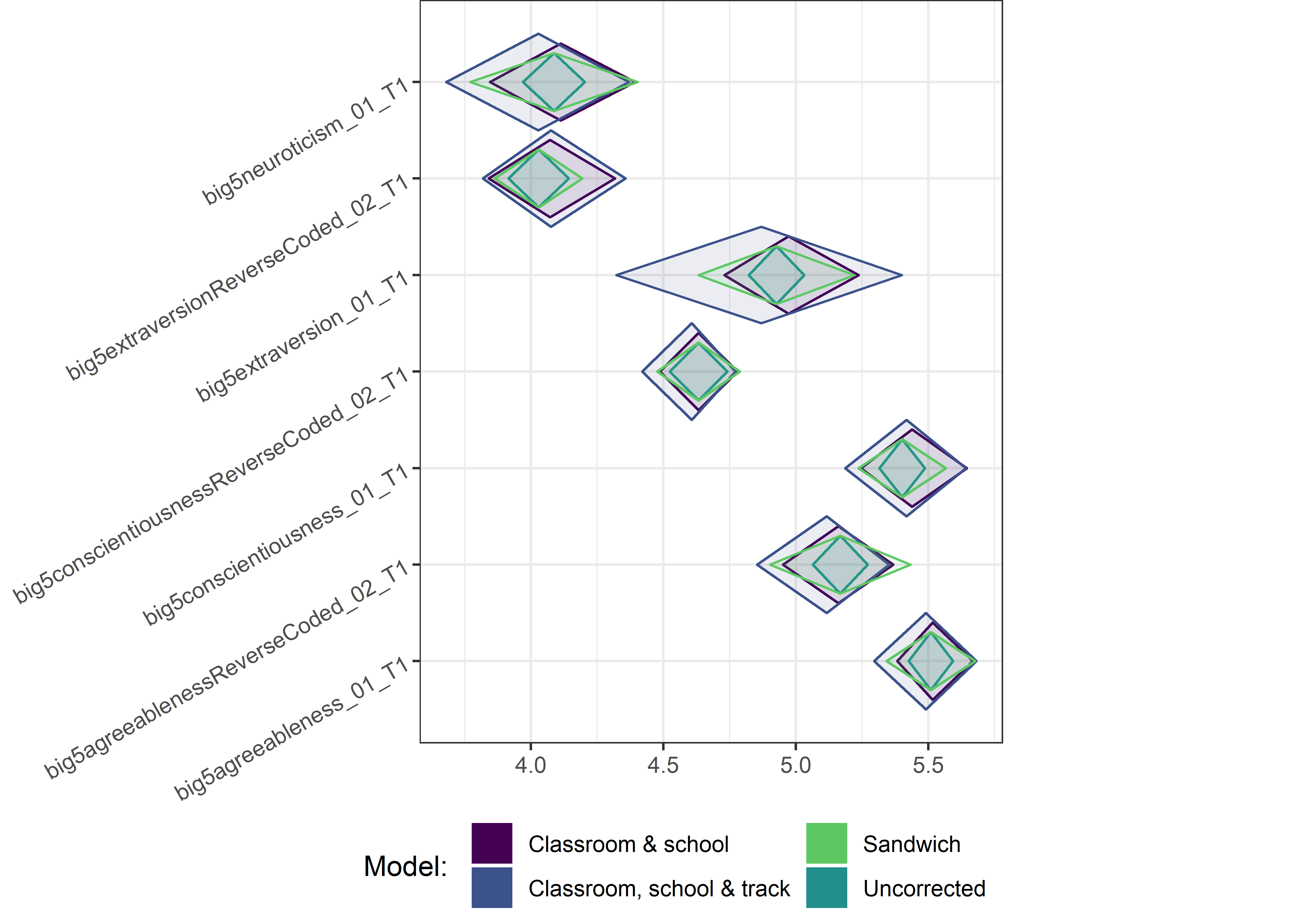
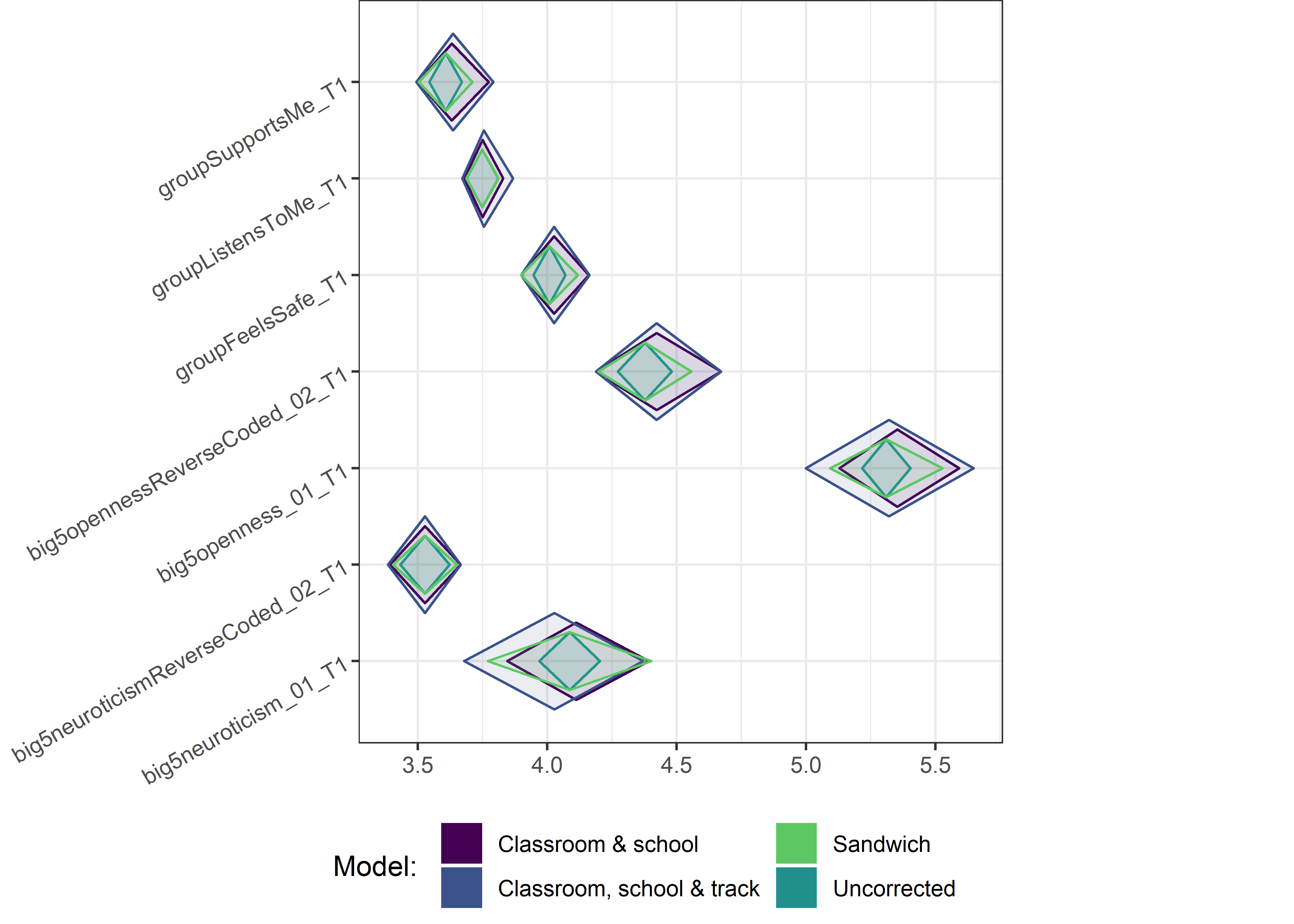
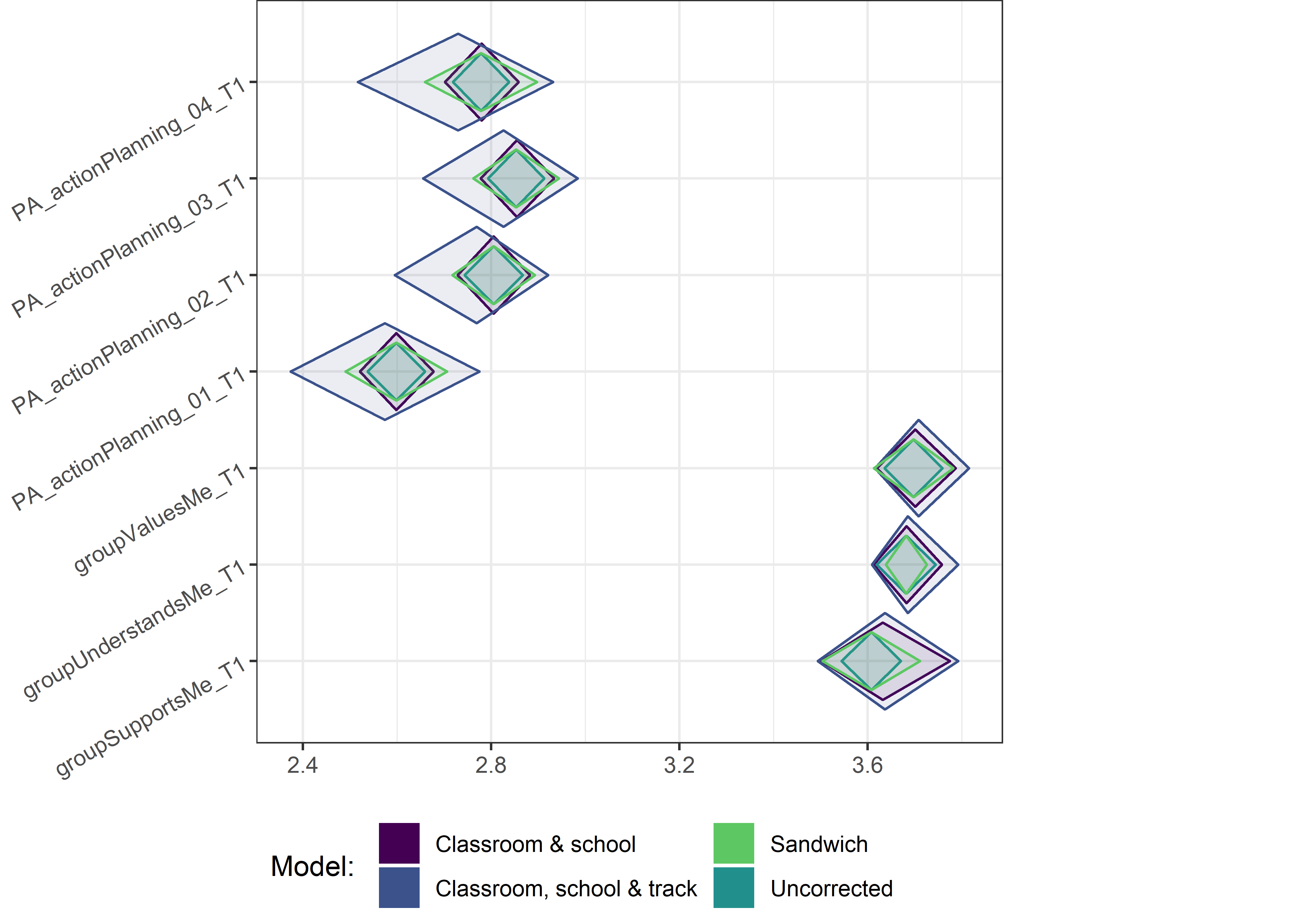
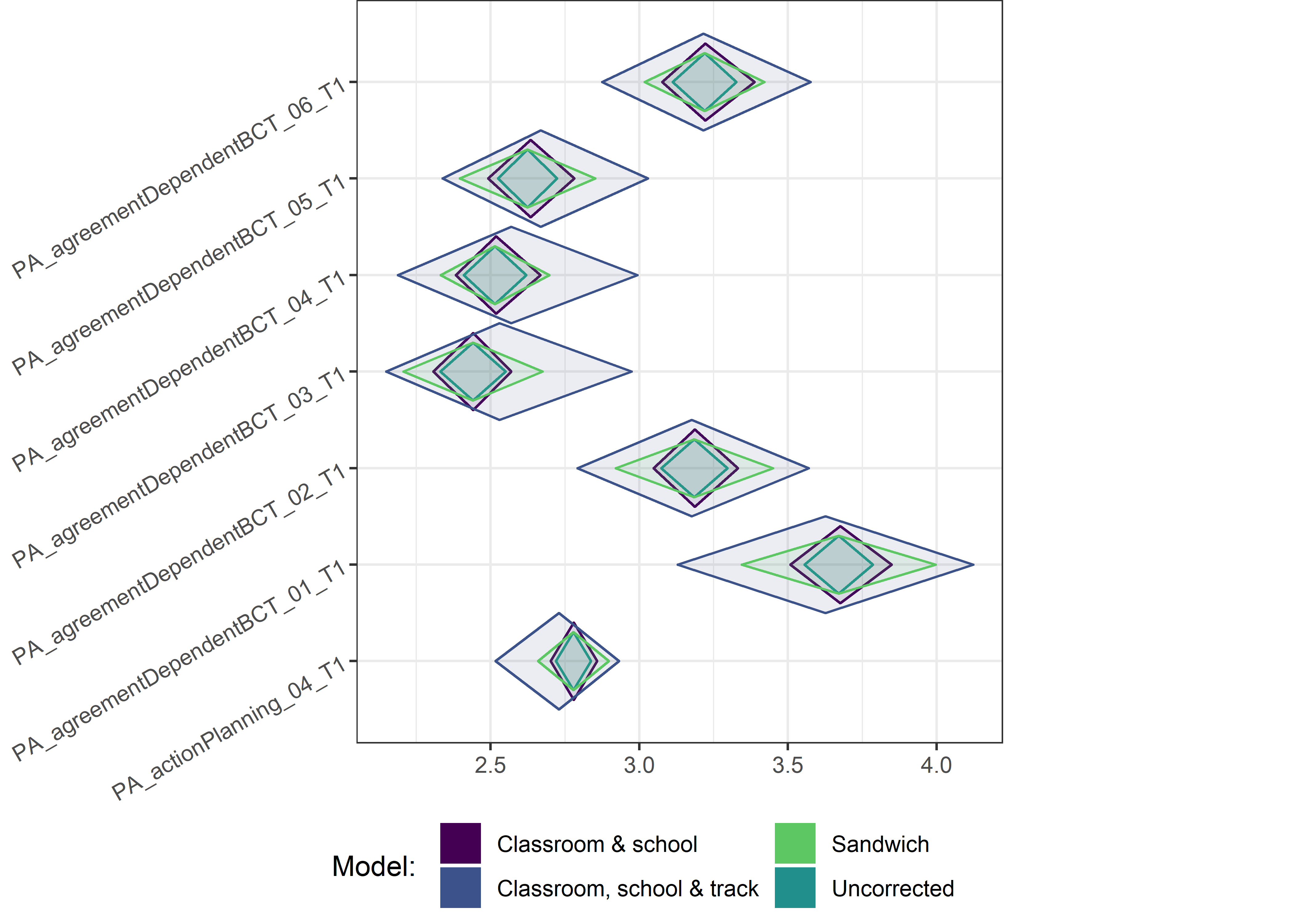
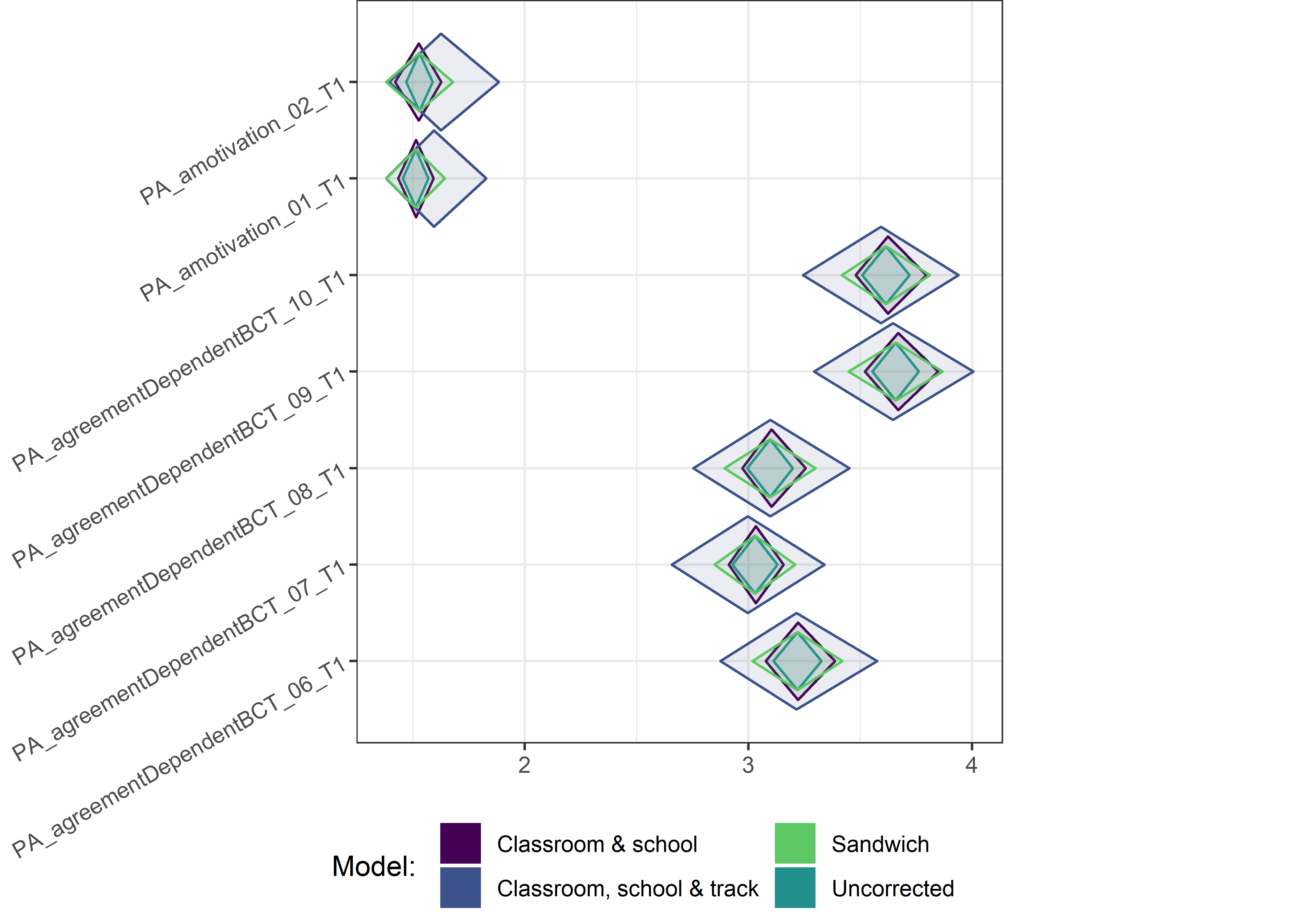
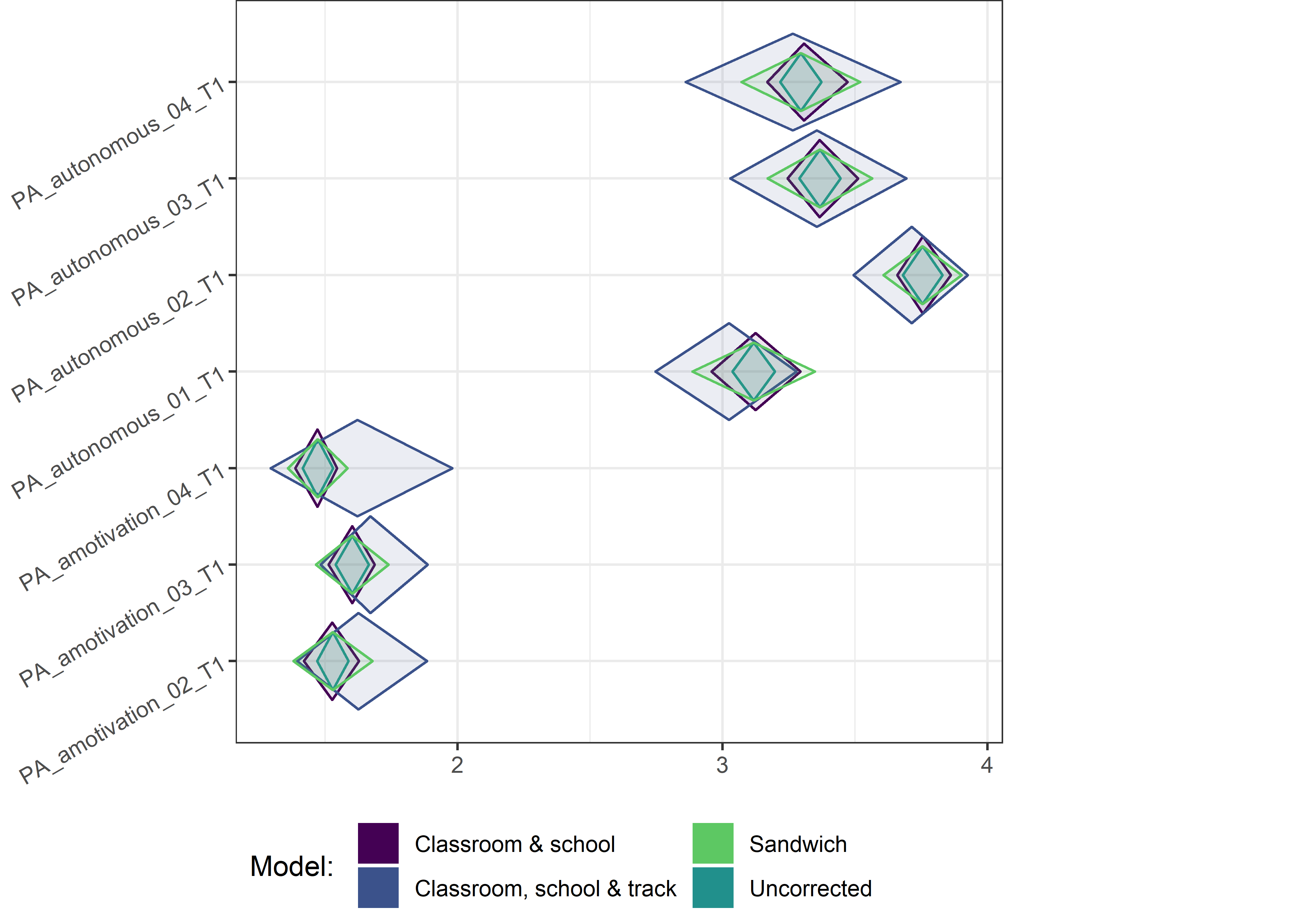
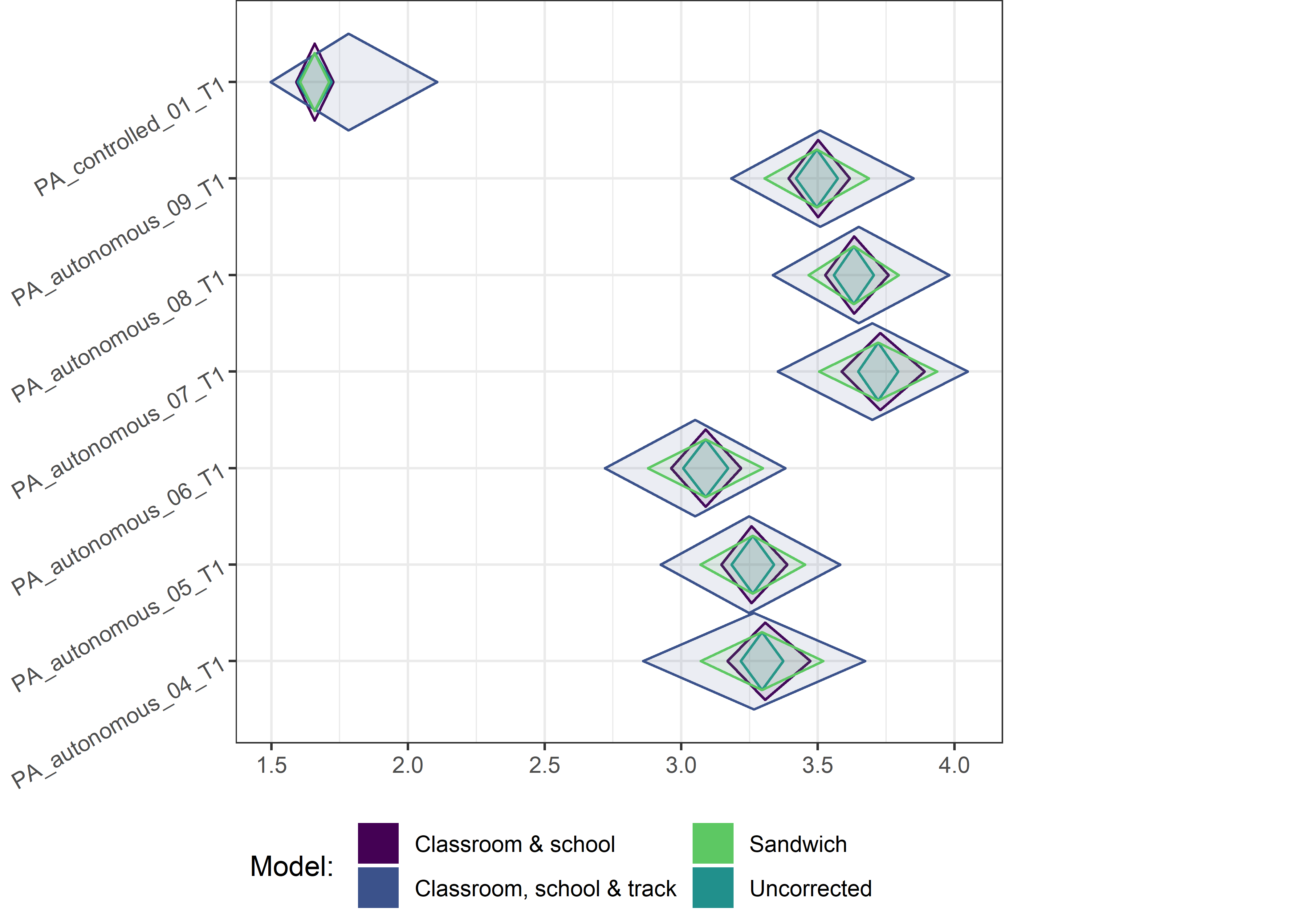
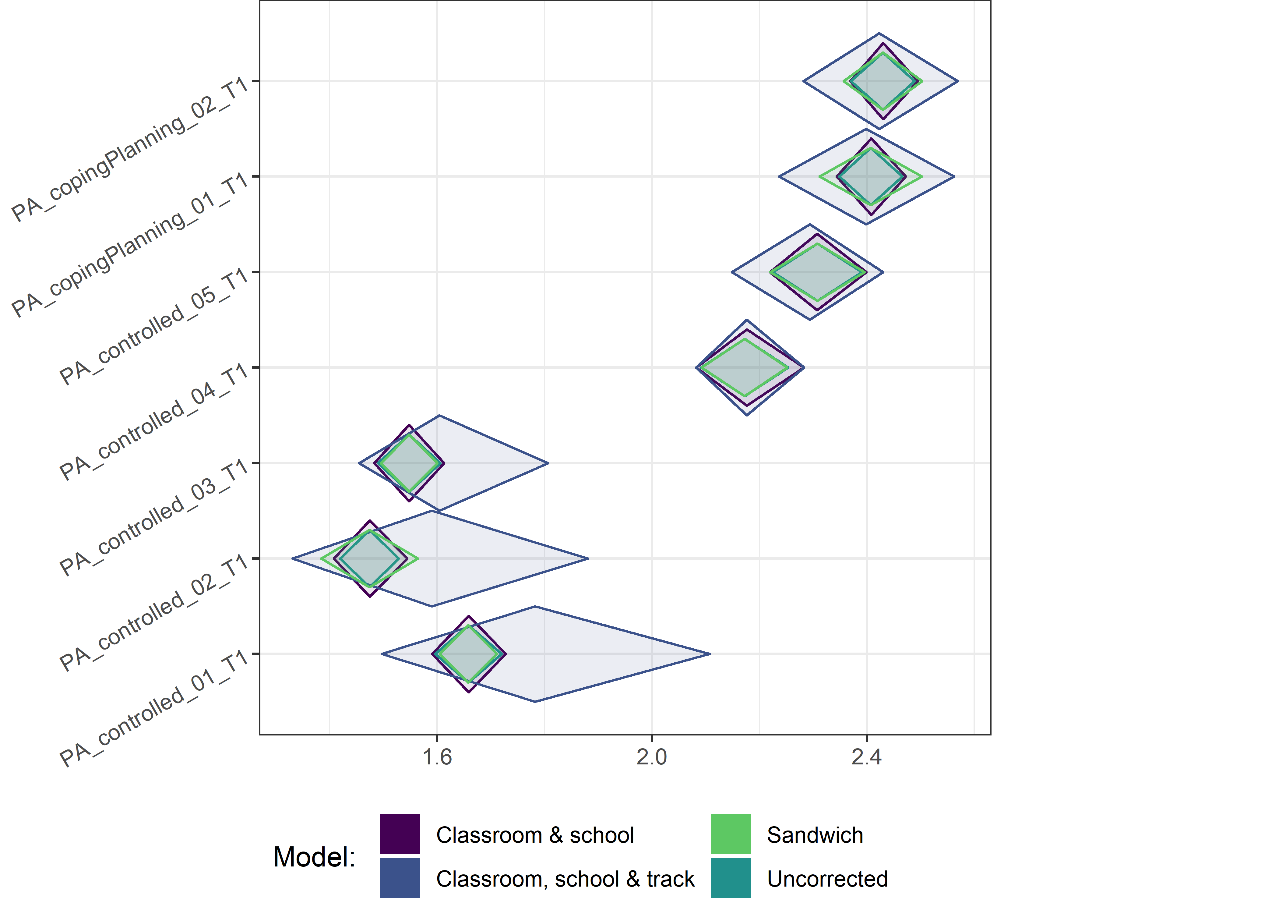
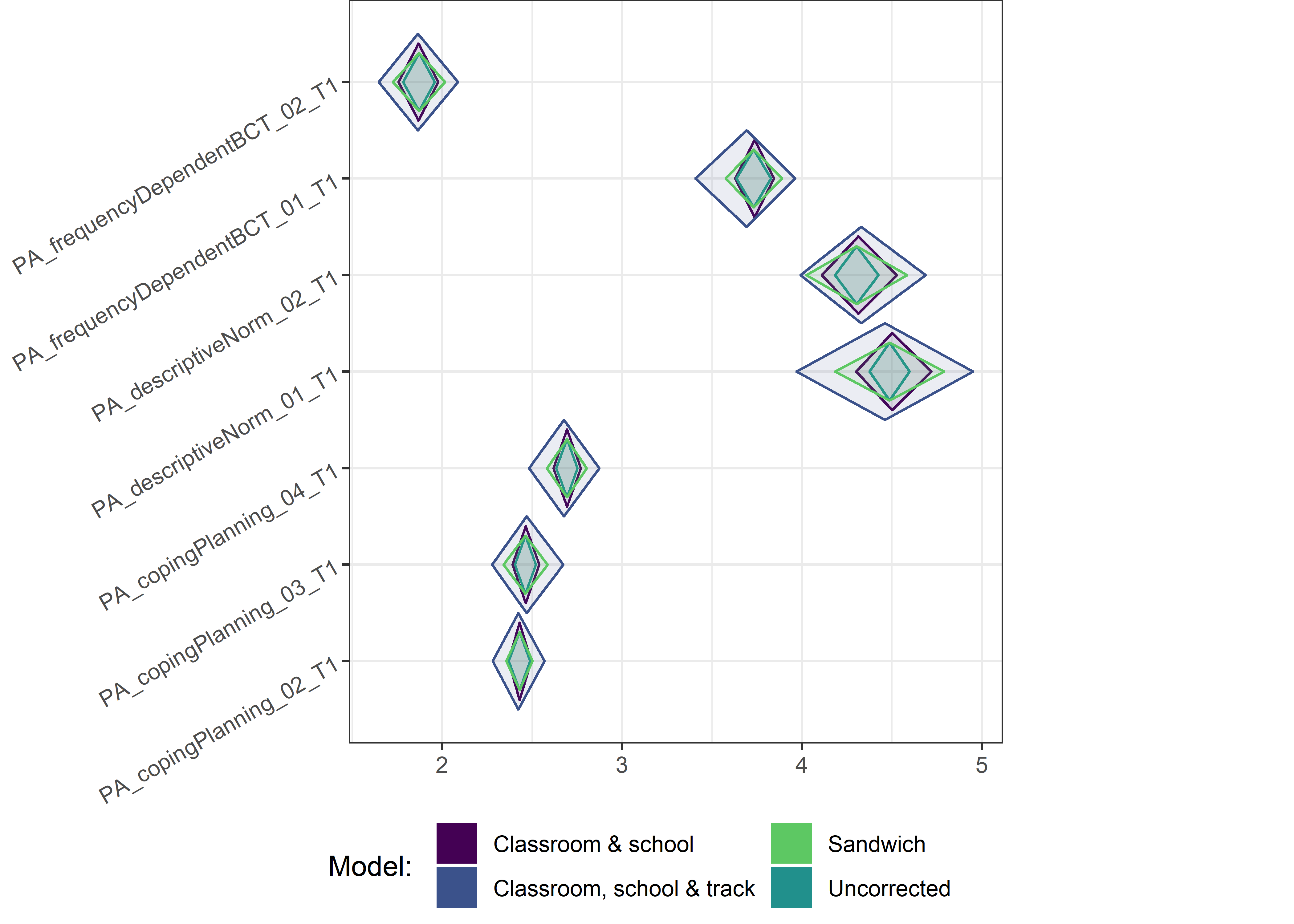
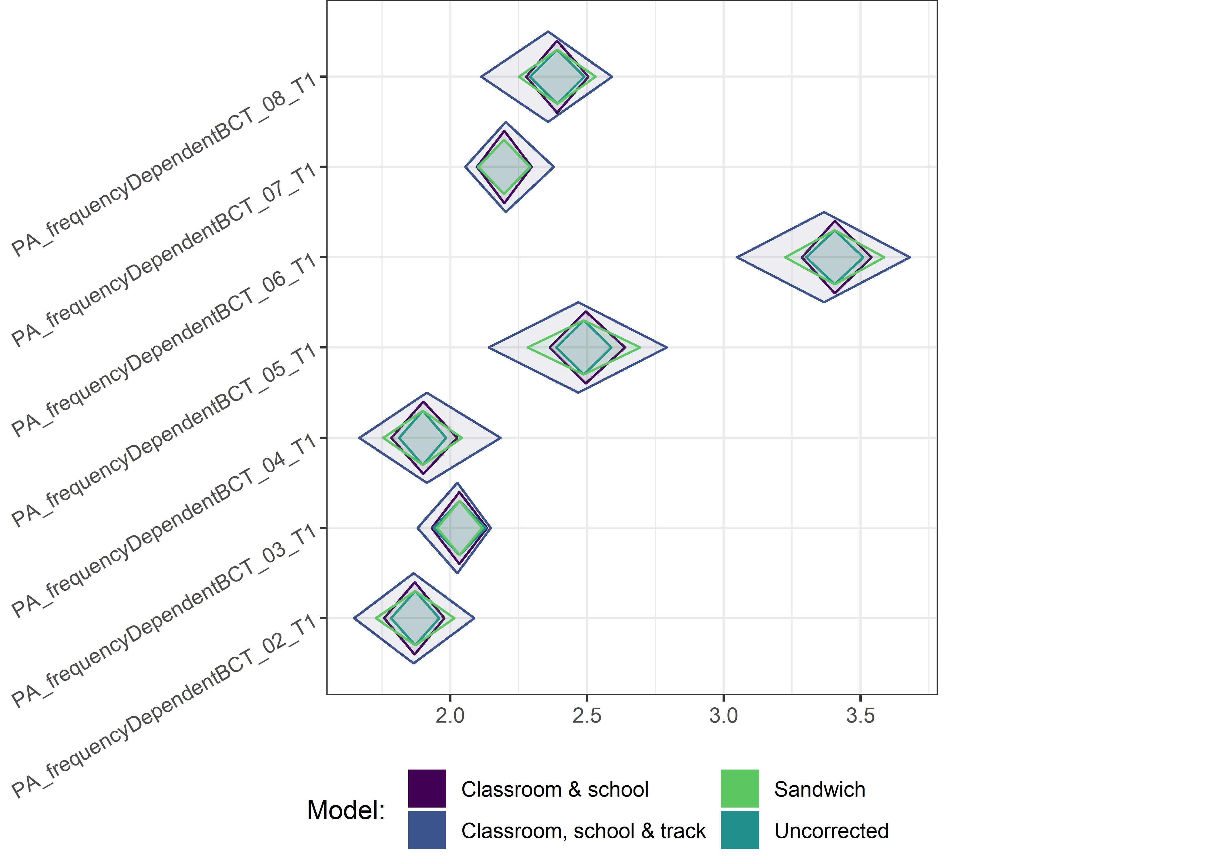
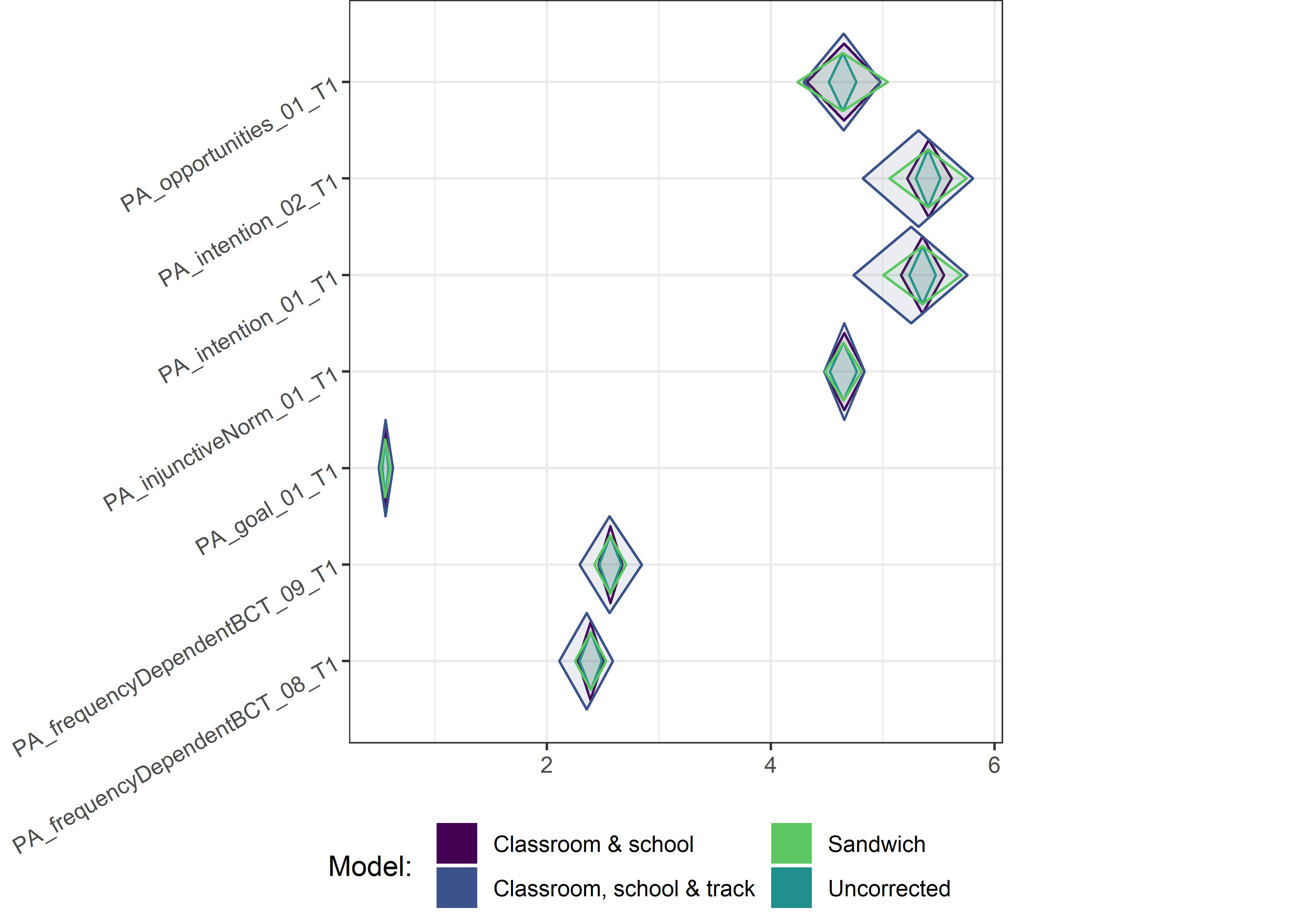
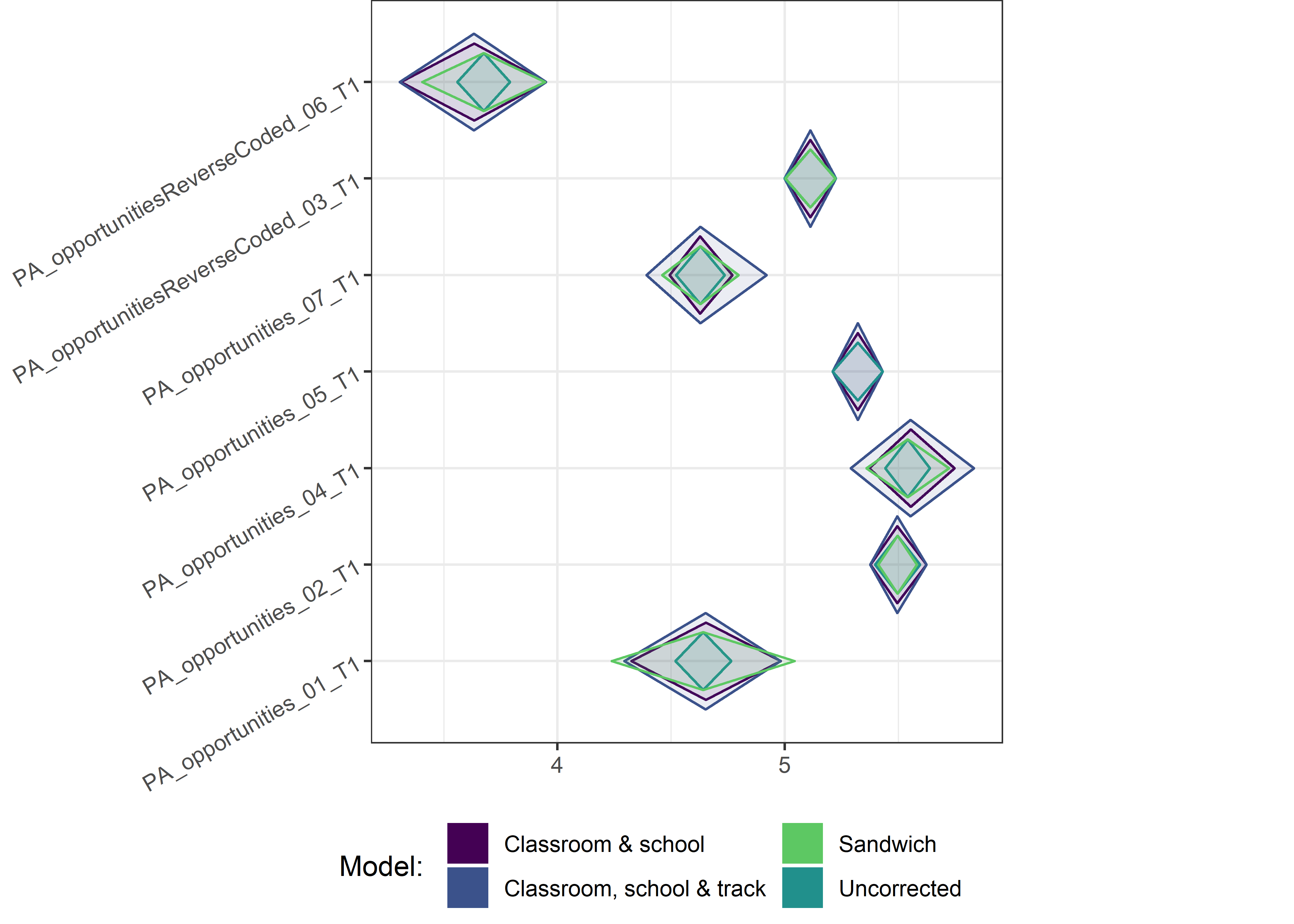
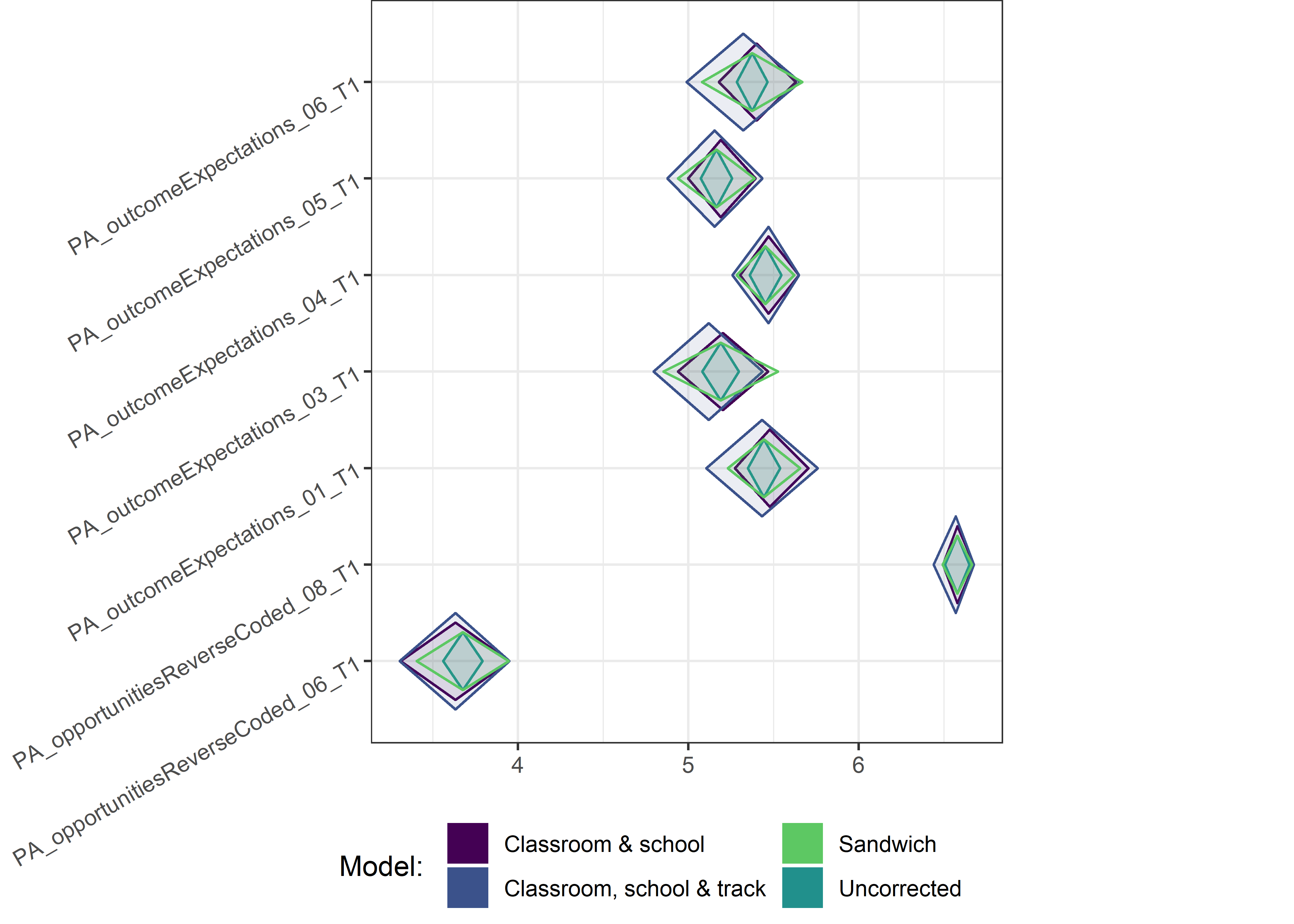
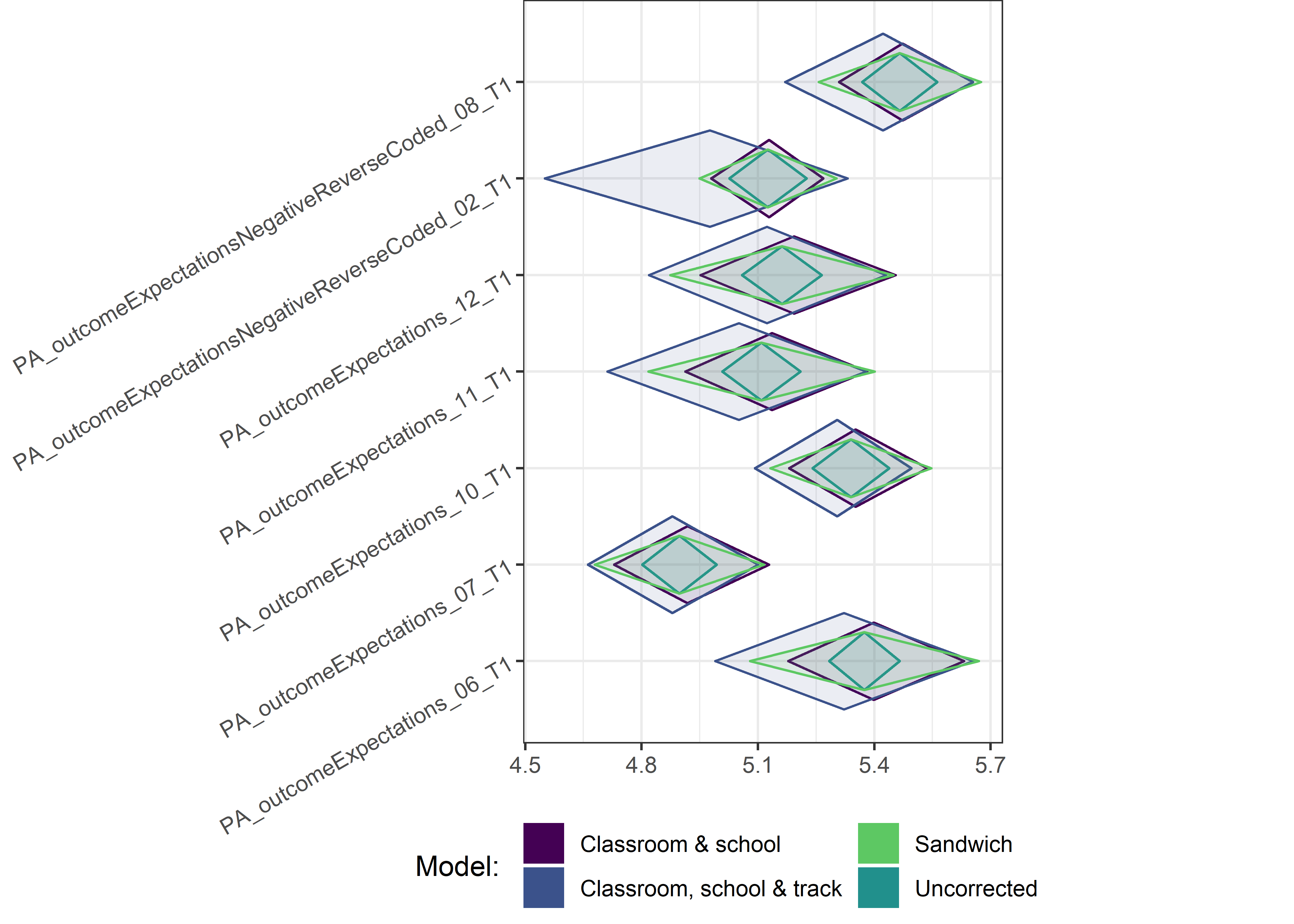
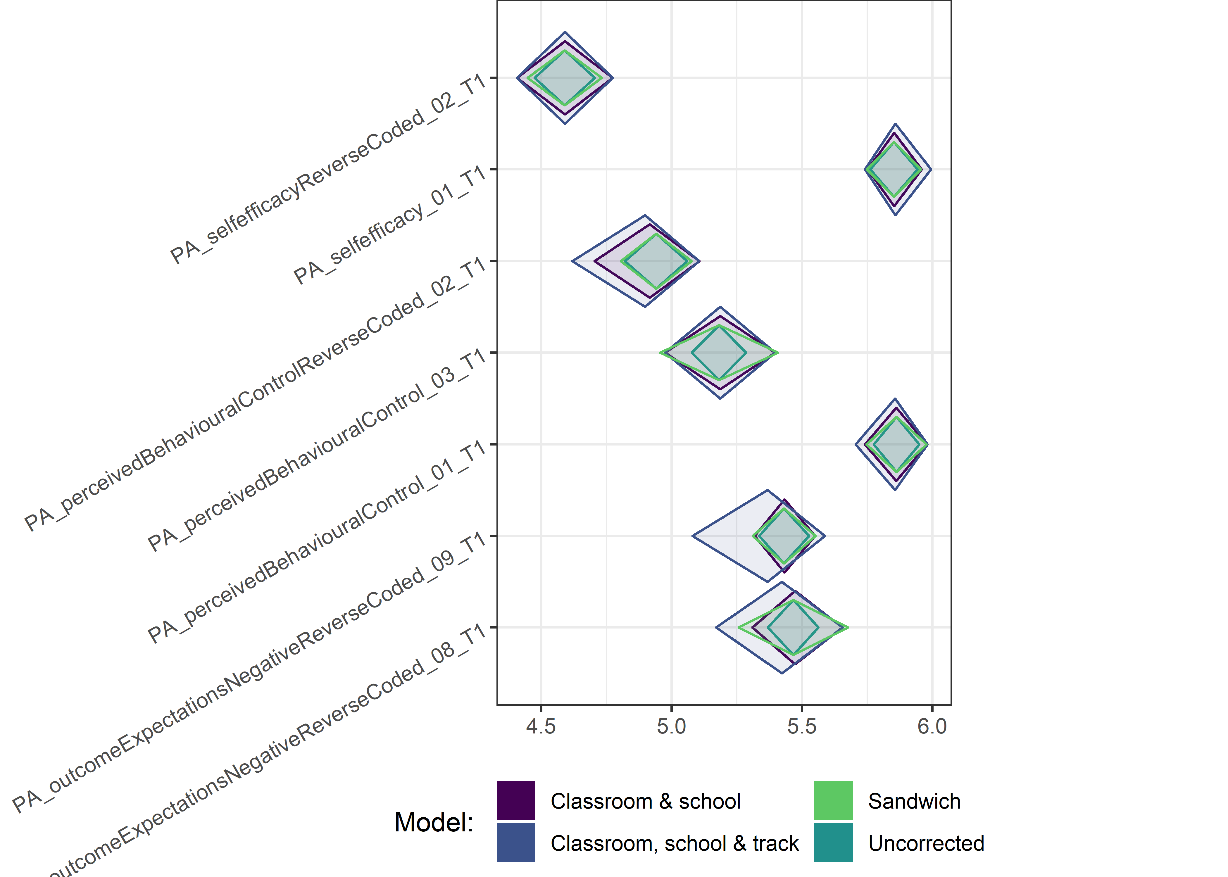
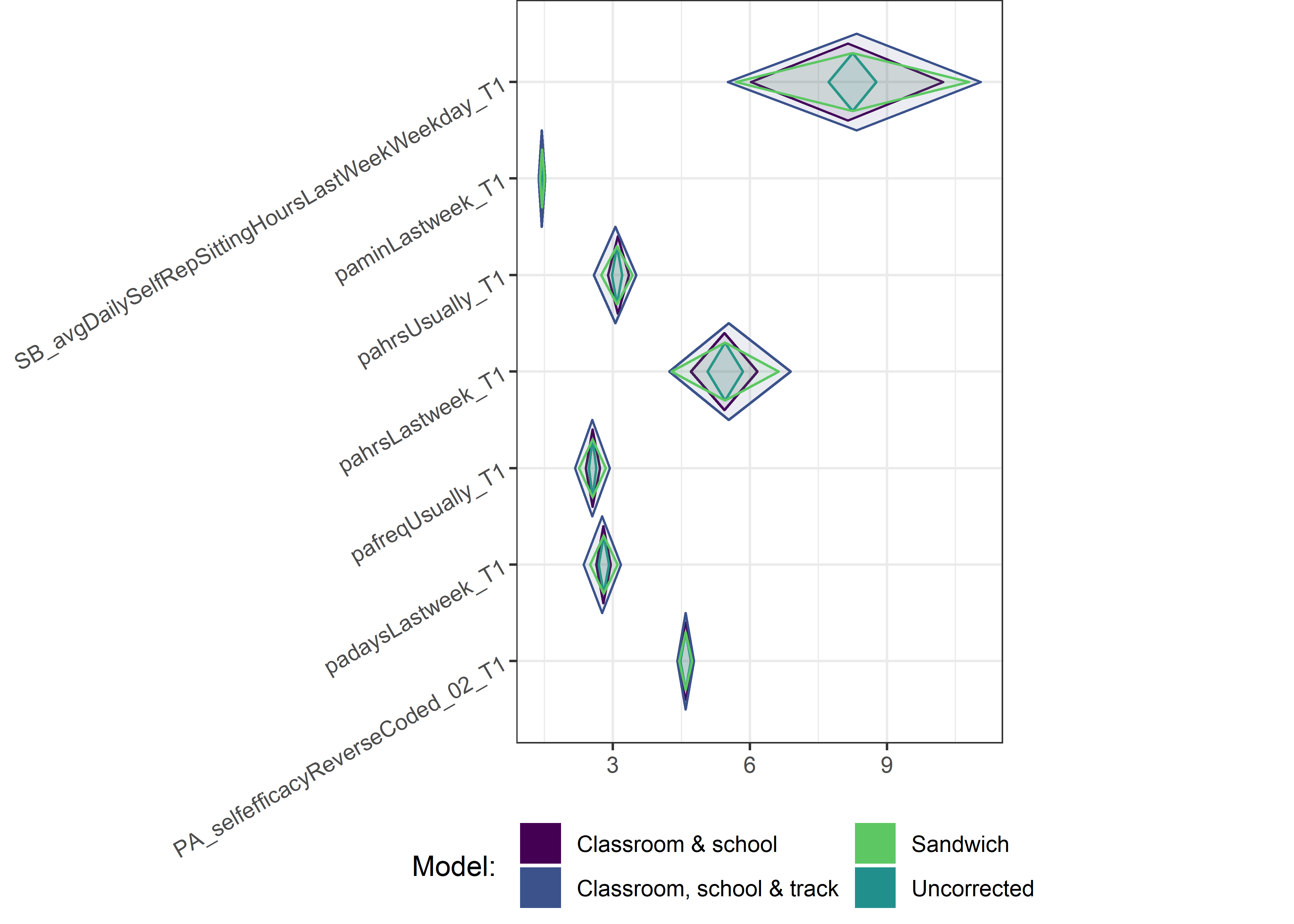
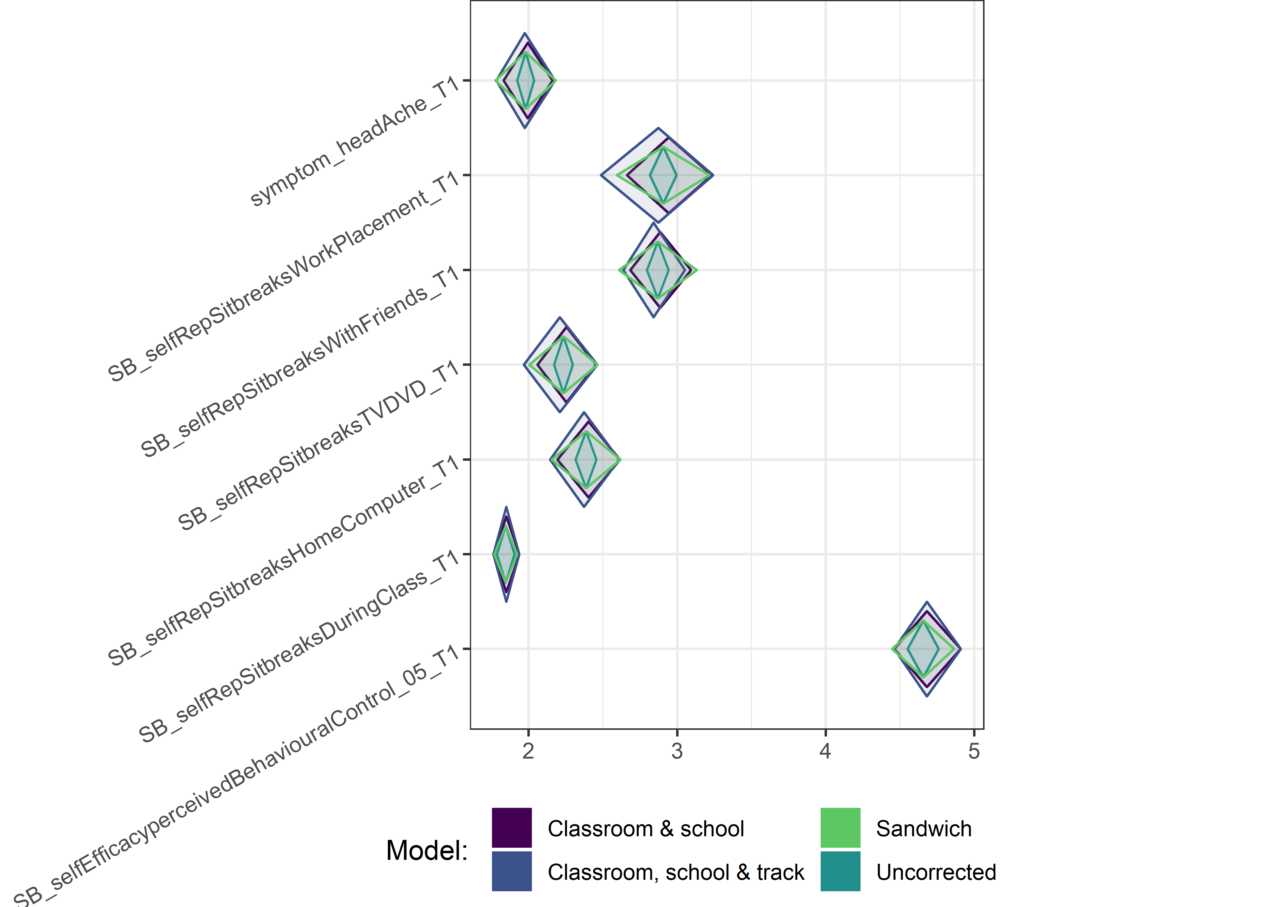
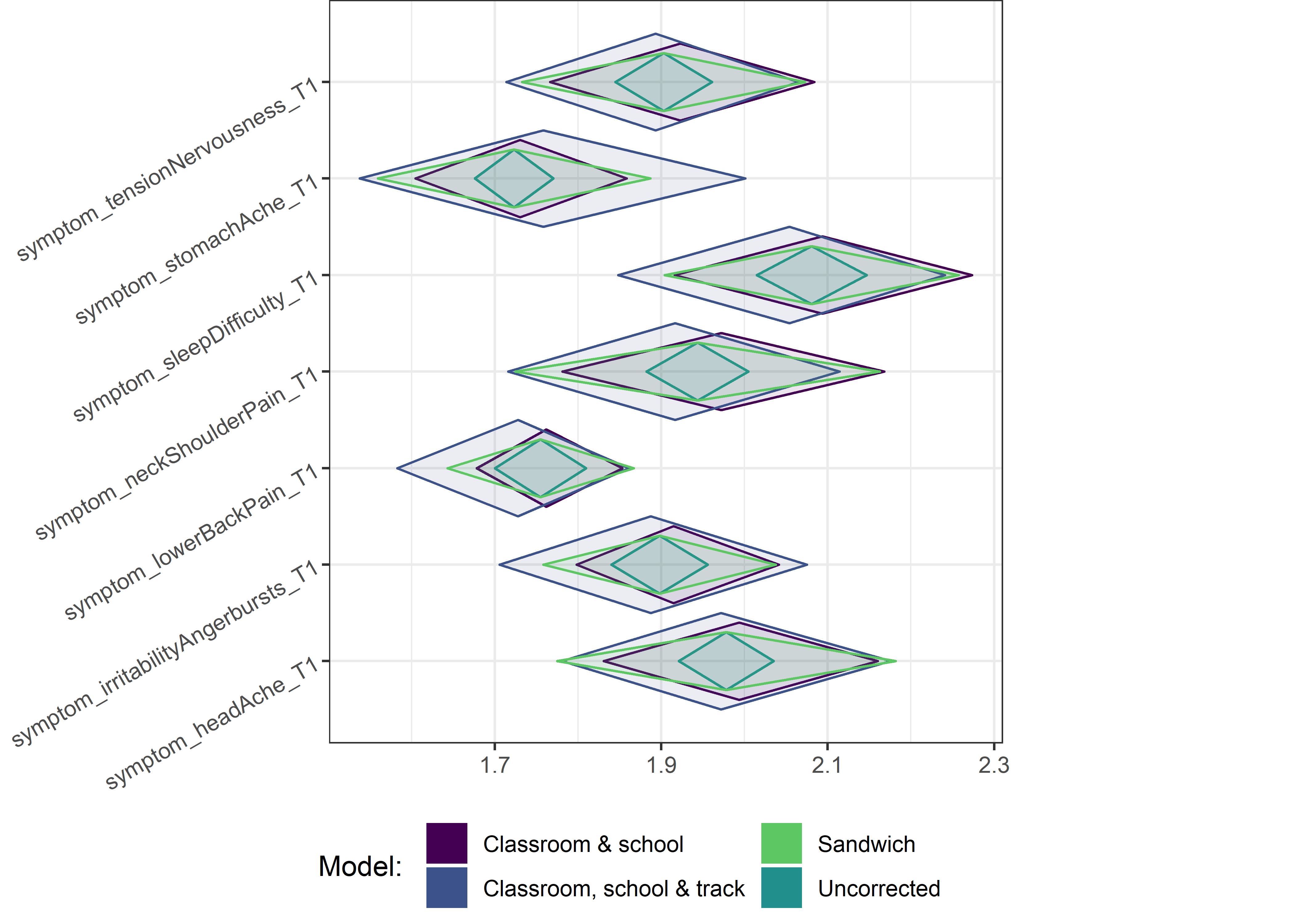
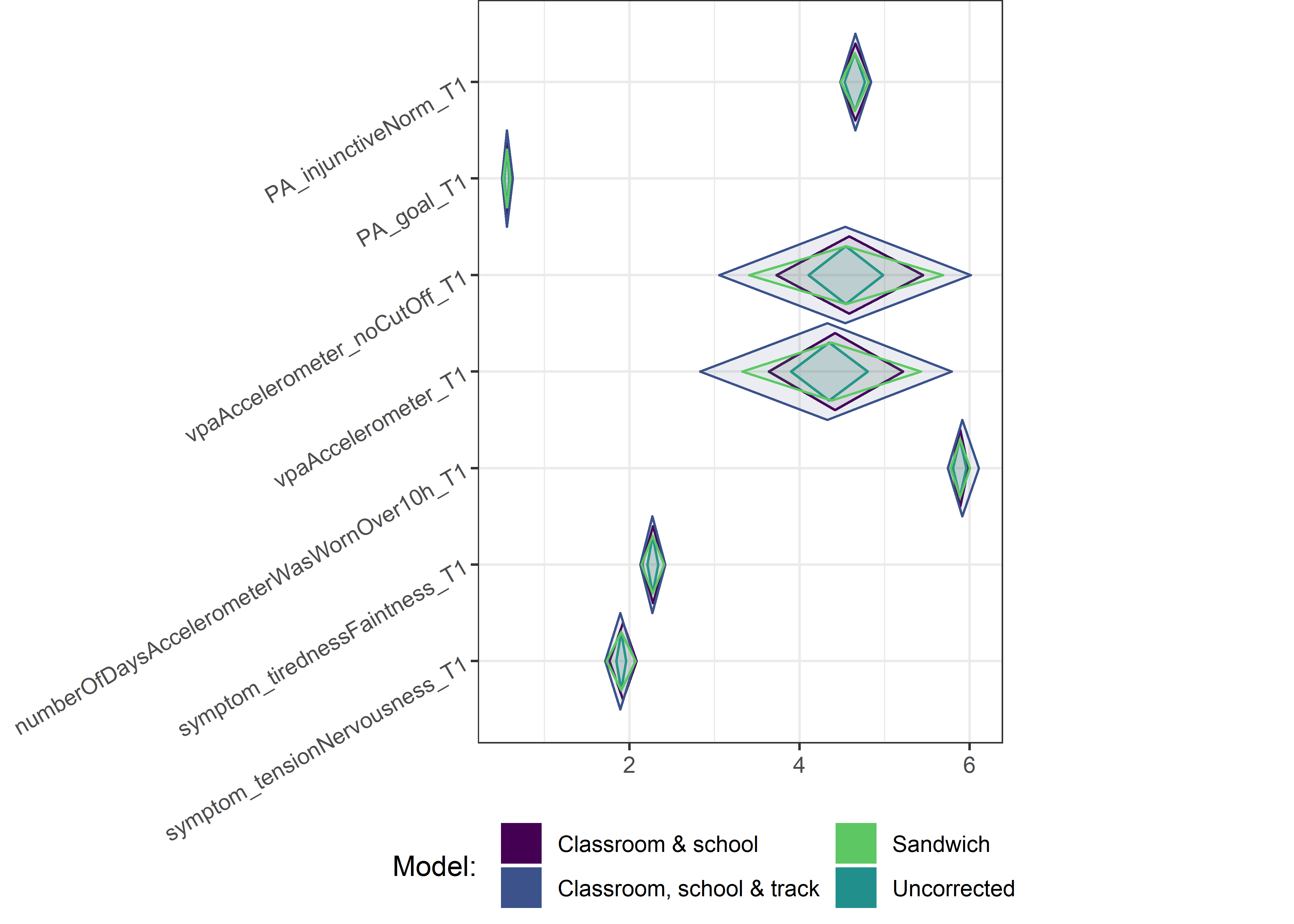
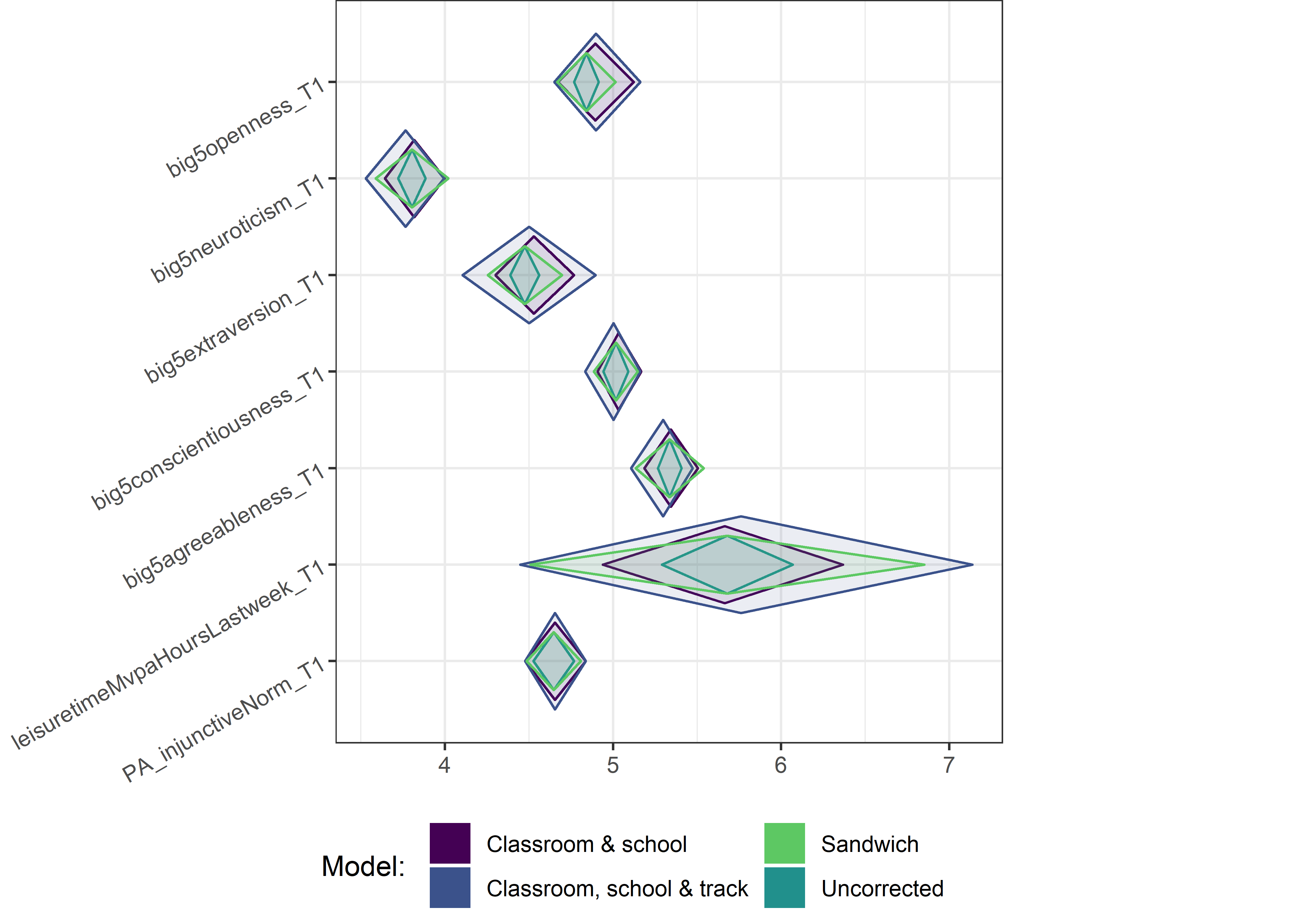
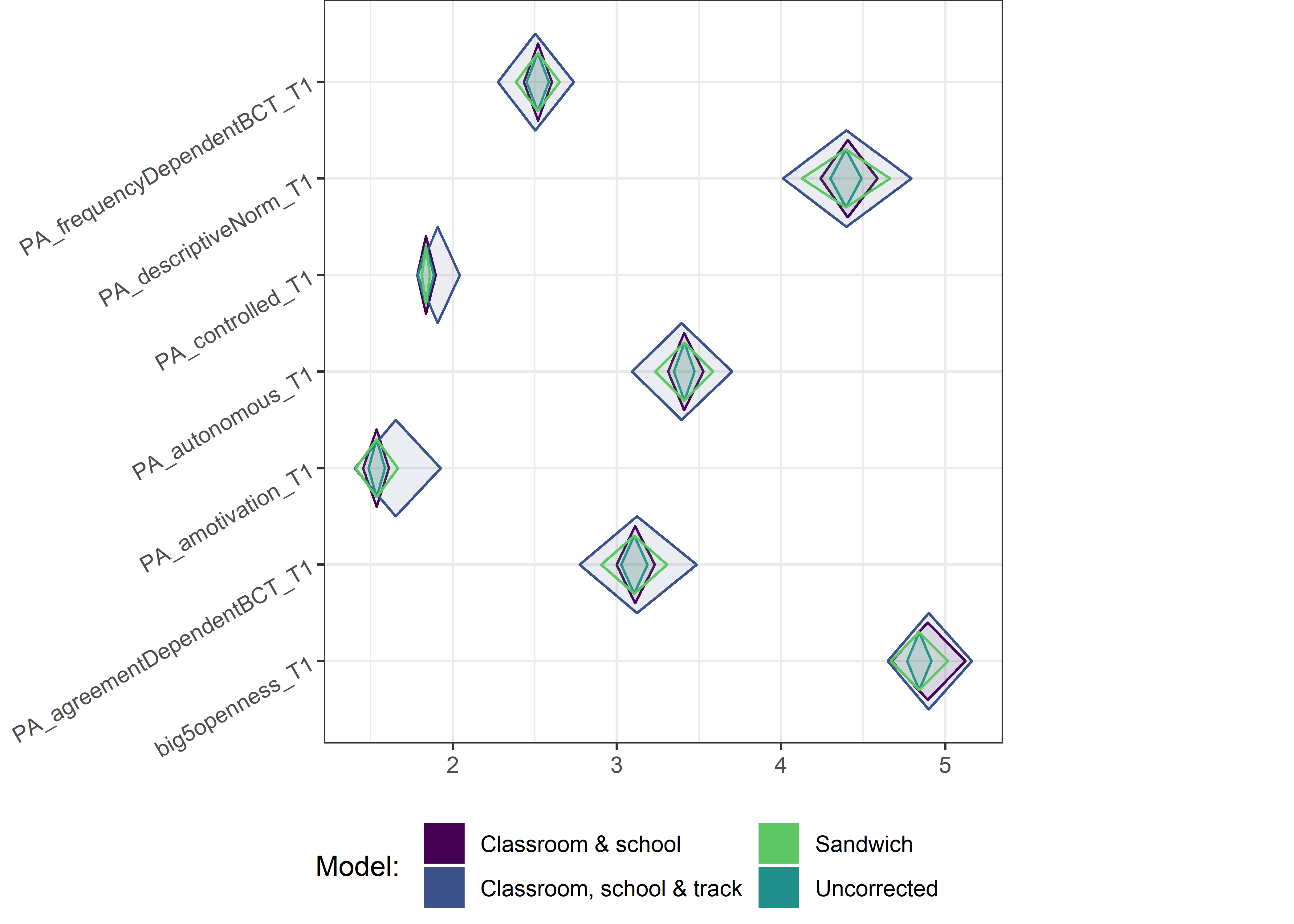
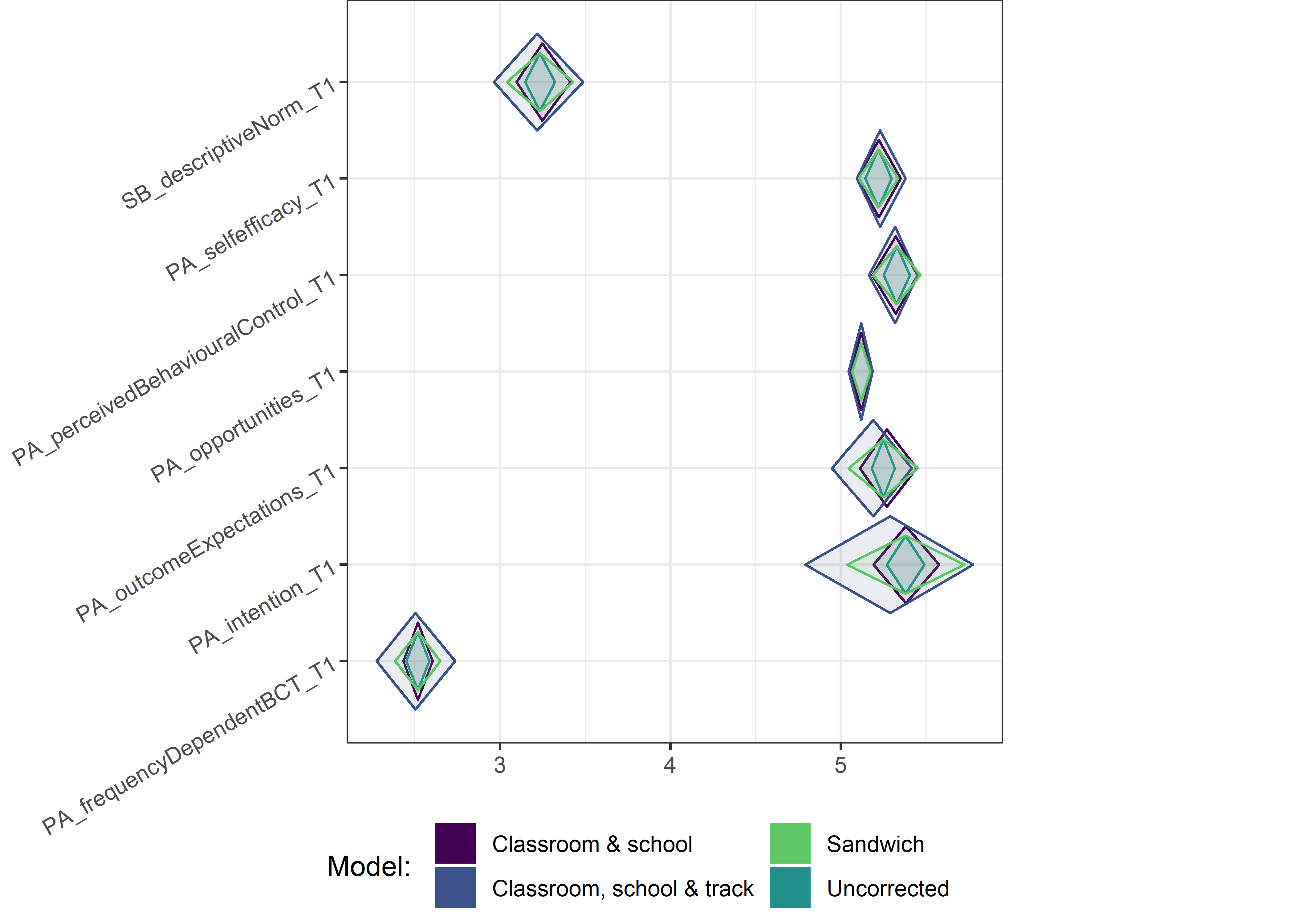
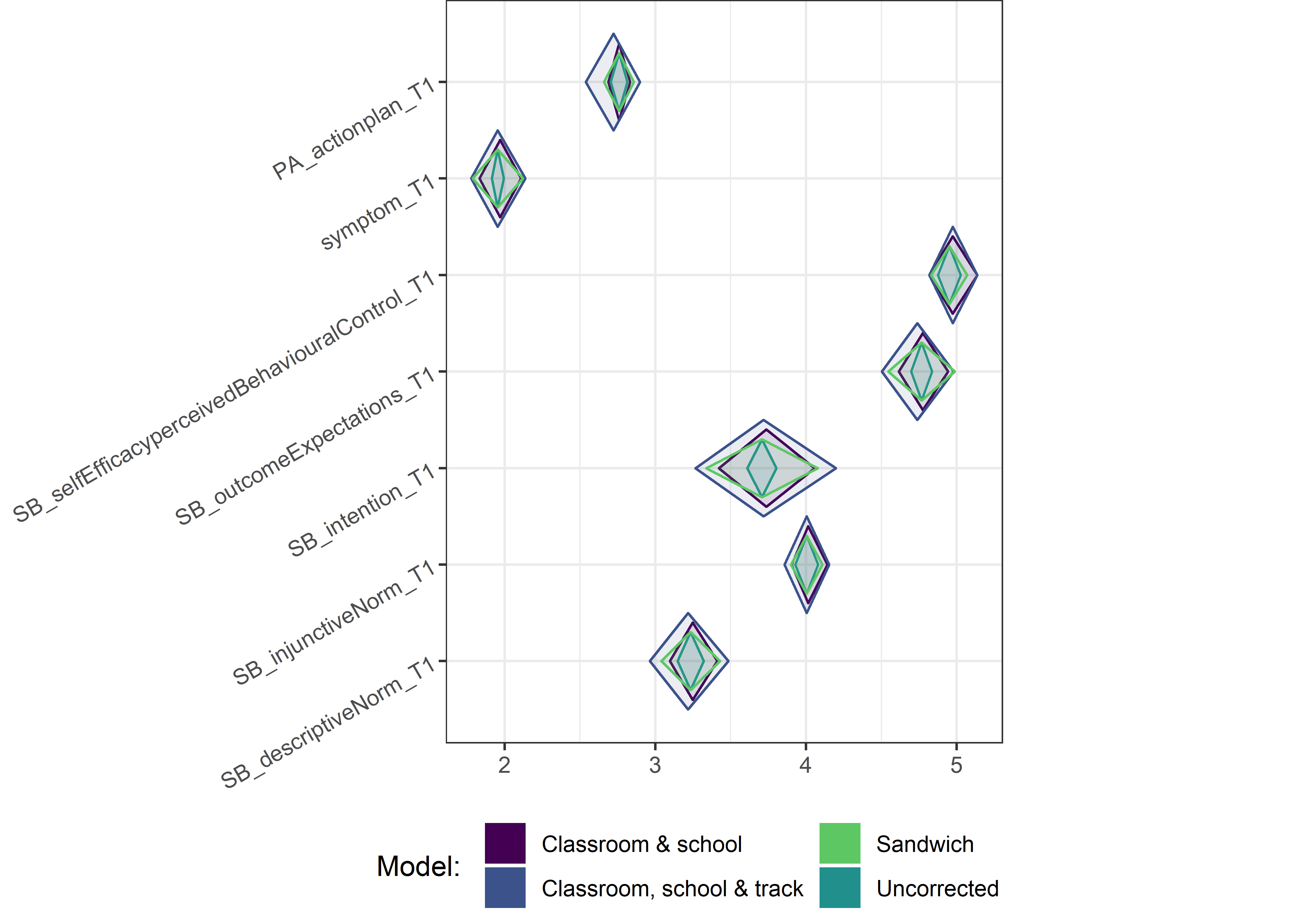
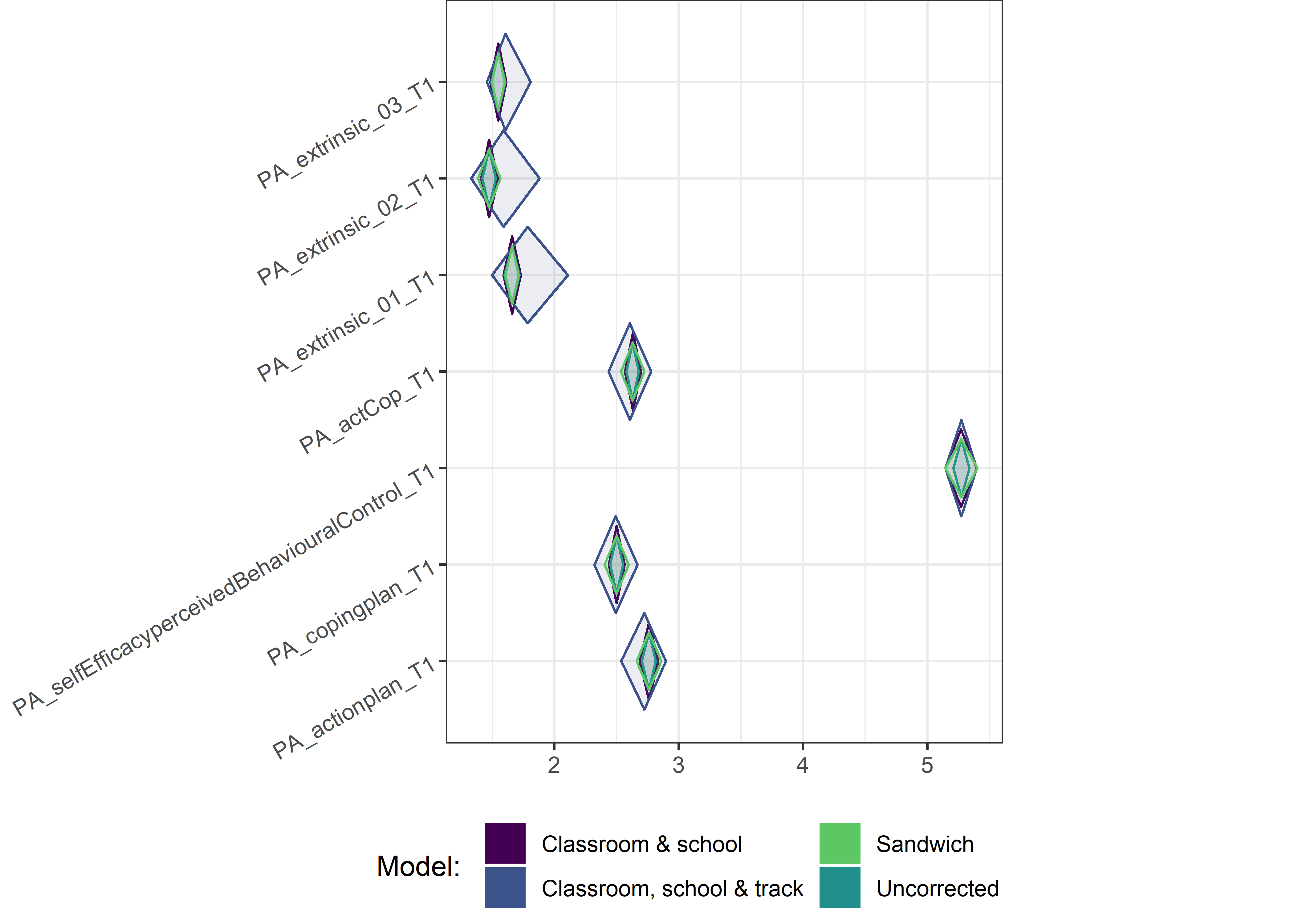
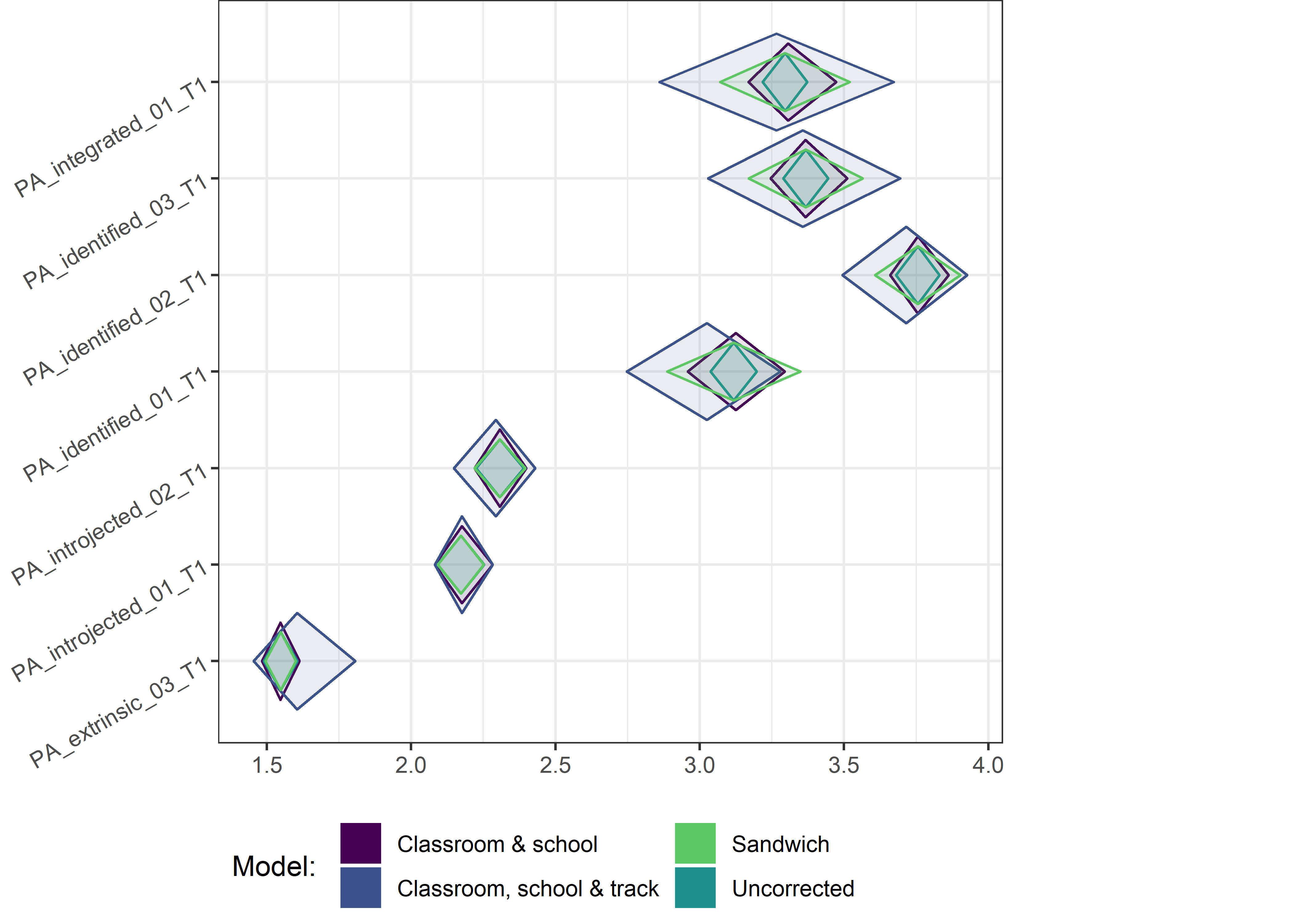
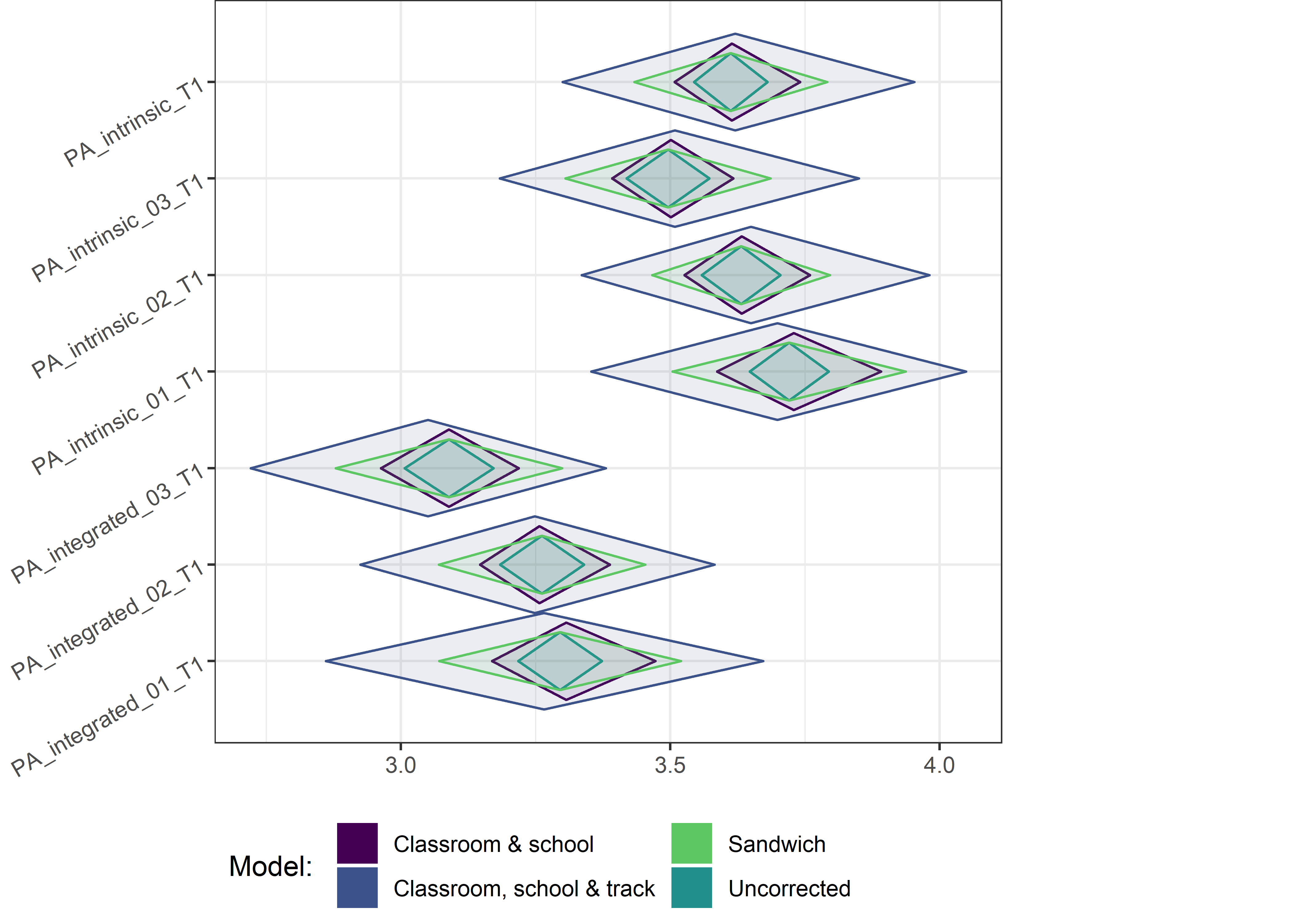
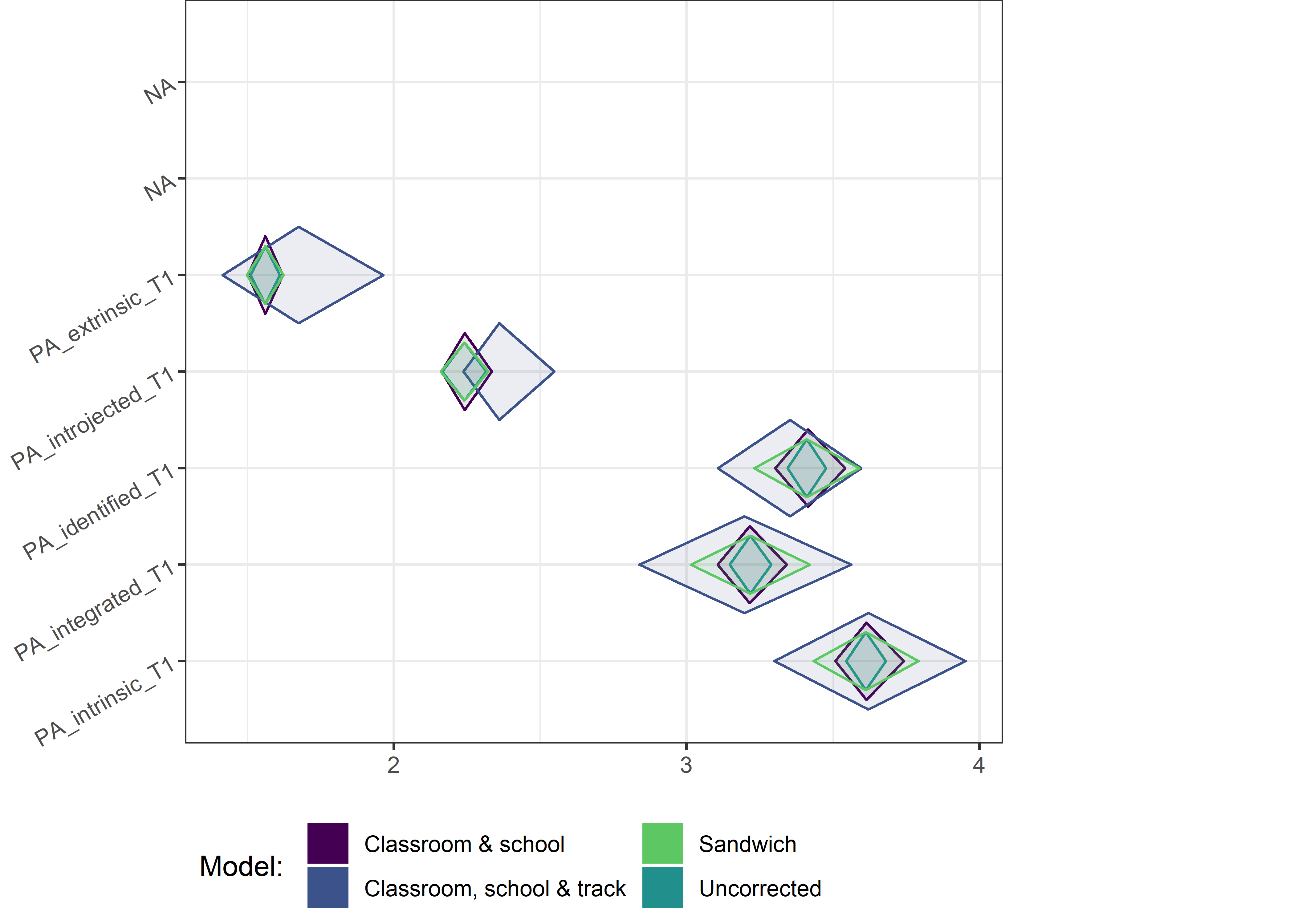
  DT::datatable()

Visual comparison of different estimates for means and CIs

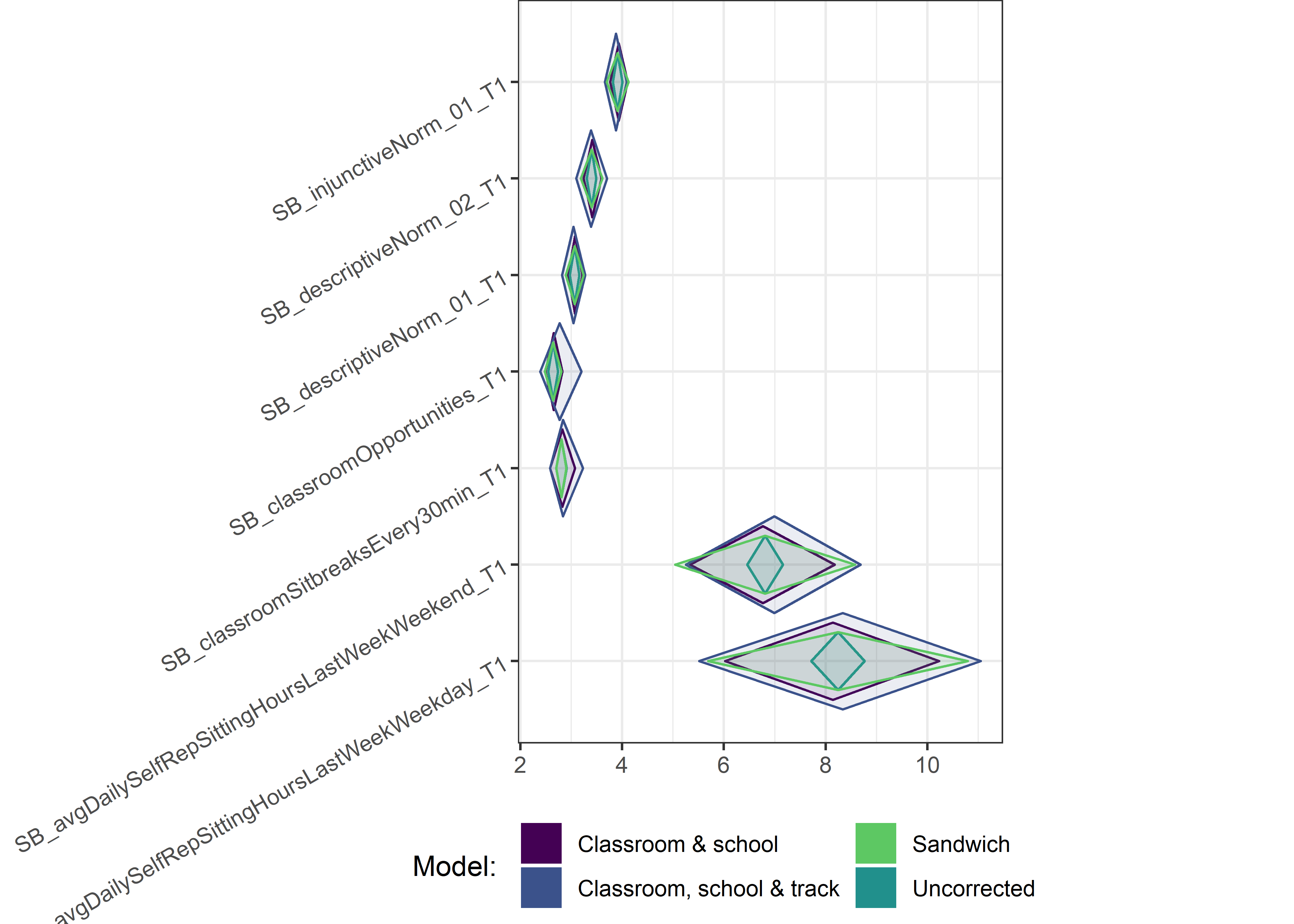
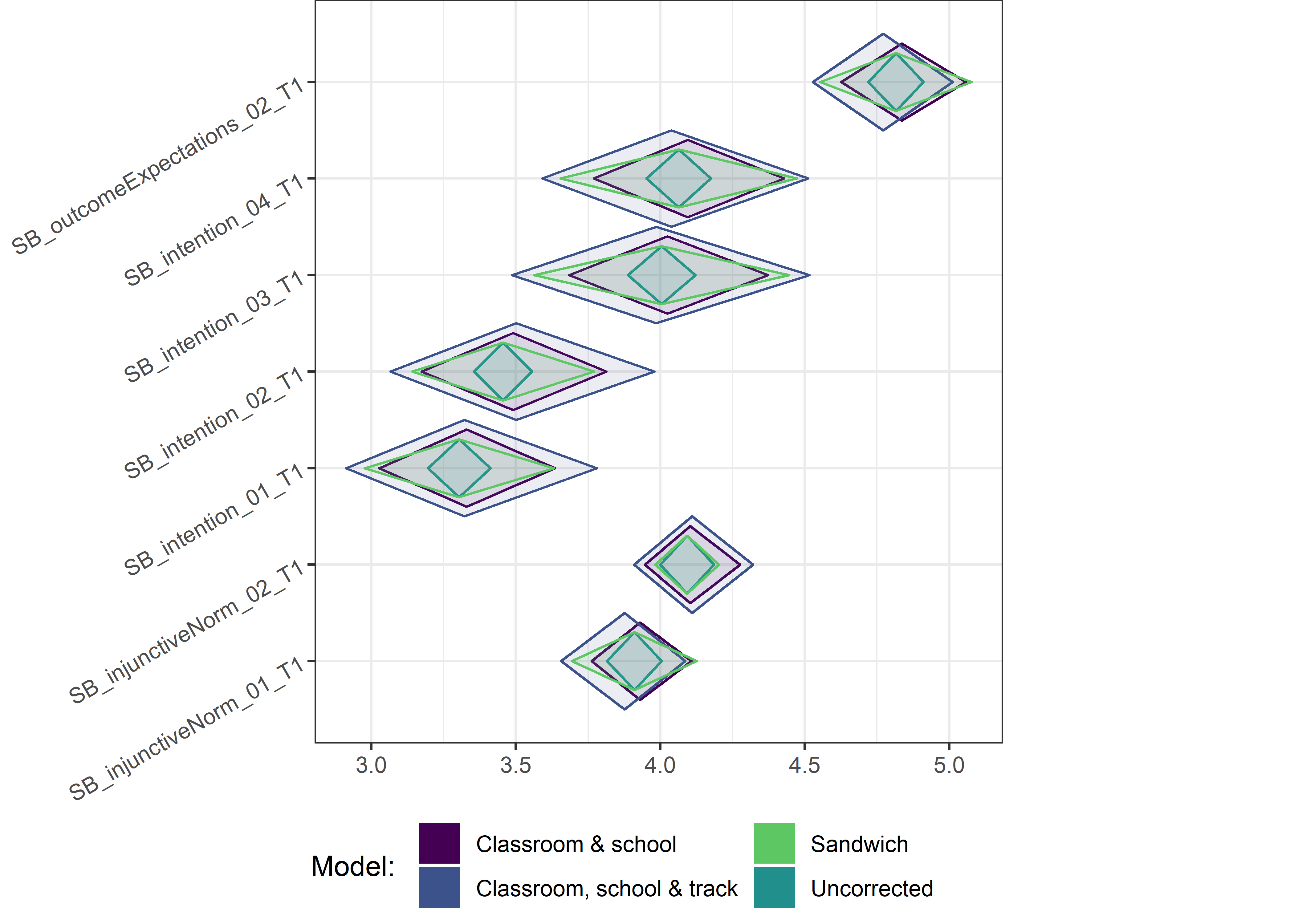
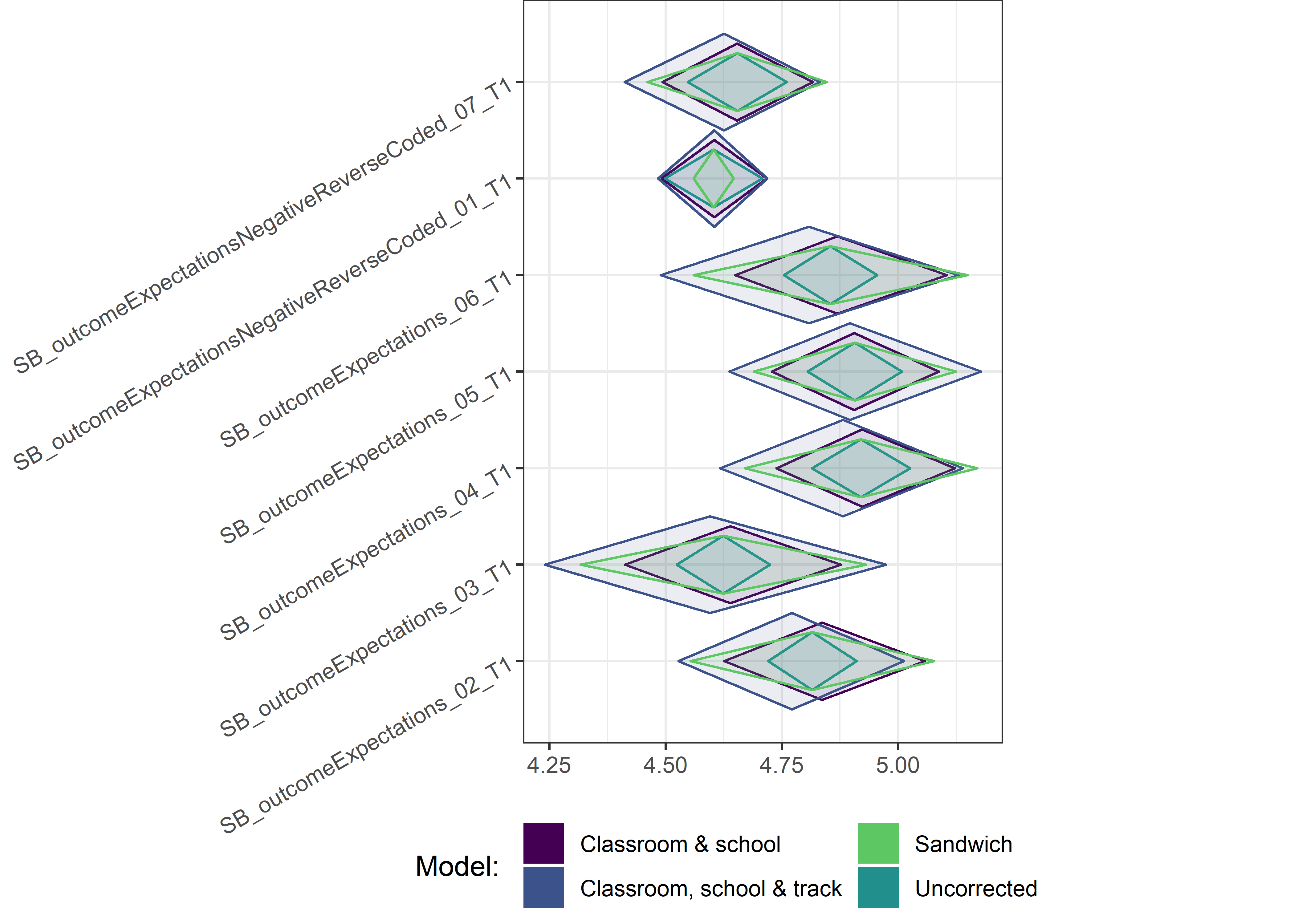
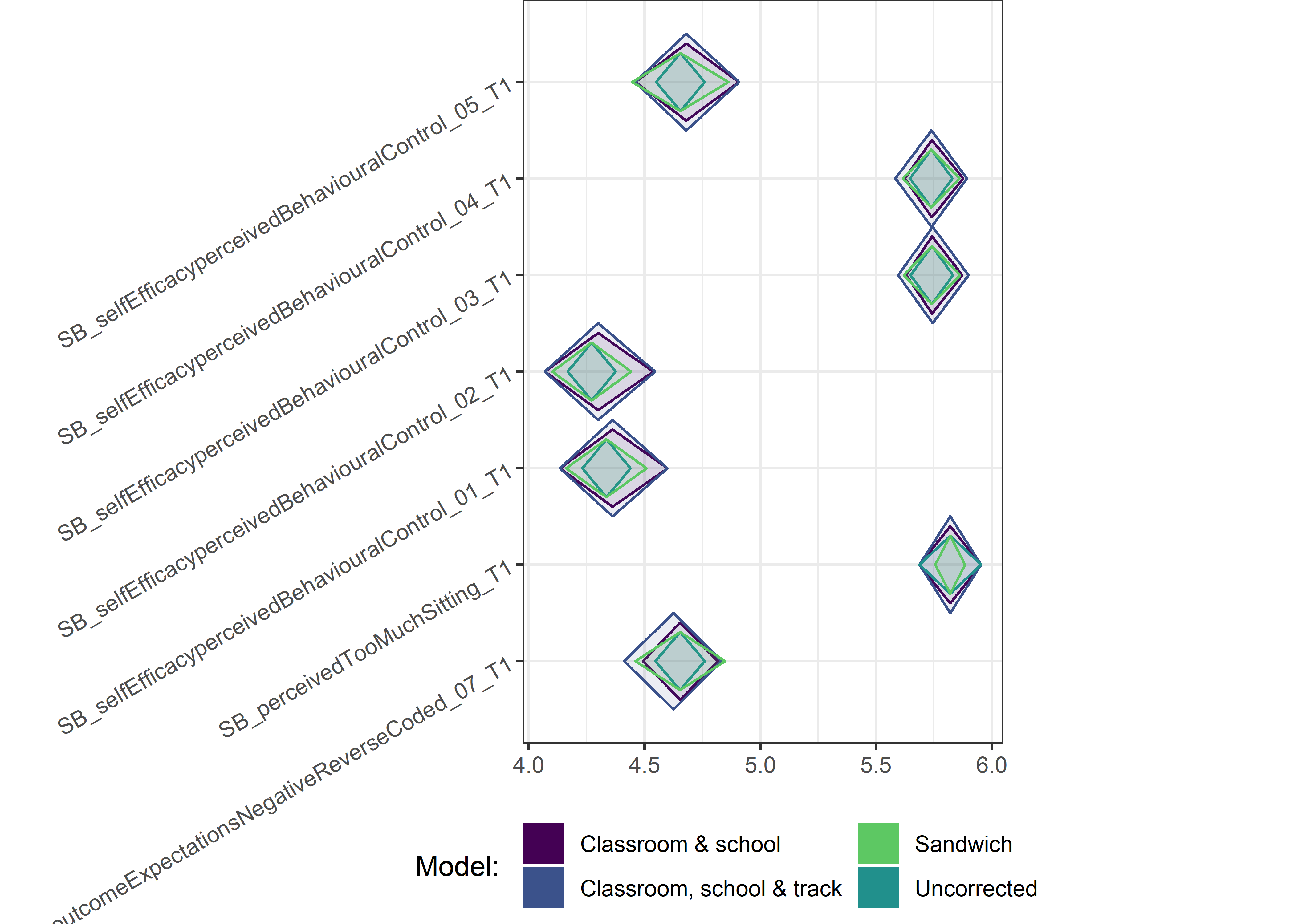
This section contains diamond plots comparing different estimates for means and CIs.

High-mean variables

ci_total_big <- ci_total %>% dplyr::filter(mean > 10)
ci_edutrack_big <- ci_edutrack %>% dplyr::filter(mean > 10)
ci_uncorrected_big <- ci_uncorrected %>% dplyr::filter(mean > 10)
ci_sandwich_big <- ci_sandwich %>% dplyr::filter(mean > 10)
# ci_bayes_big <- ci_bayes %>% dplyr::filter(mean > 10)
# ci_bayes_containing_edutrack_big <- ci_bayes_containing_edutrack %>% dplyr::filter(mean > 10)

for (i in 1:4){
plot1 <- userfriendlyscience::diamondPlot(ci_total_big[i, ], 
                                          color = viridis::viridis(5)[1], 
                                          alpha = 0.1, 
                                          yLabels = ci_total_big[i, ]$diamondlabels, 
                                          fixedSize = 0.4, 
                                          xlab = NULL) +
  userfriendlyscience::diamondPlot(ci_edutrack_big[i, ], 
                                   returnLayerOnly = TRUE,
                                   color = viridis::viridis(5)[2], 
                                   alpha = 0.1, 
                                   yLabels = ci_edutrack_big[i, ]$diamondlabels, 
                                   fixedSize = 0.5, 
                                   xlab = NULL) +
  userfriendlyscience::diamondPlot(ci_uncorrected_big[i, ], 
                                   returnLayerOnly = TRUE,
                                   color = viridis::viridis(5)[3], 
                                   alpha = 0.1, 
                                   yLabels = ci_uncorrected_big[i, ]$diamondlabels, 
                                   fixedSize = 0.3, 
                                   xlab = NULL) +
  userfriendlyscience::diamondPlot(ci_sandwich_big[i, ], 
                                   returnLayerOnly = TRUE,
                                   color = viridis::viridis(5)[4], 
                                   alpha = 0.1, 
                                   yLabels = ci_uncorrected_big[i, ]$diamondlabels, 
                                   fixedSize = 0.3, 
                                   xlab = NULL) +
  # userfriendlyscience::diamondPlot(ci_bayes_big[i, ], 
  #                                  returnLayerOnly = TRUE,
  #                                  color = "red", 
  #                                  alpha = 0, 
  #                                  yLabels = ci_uncorrected_big[i, ]$diamondlabels, 
  #                                  fixedSize = 0.10, 
  #                                  xlab = NULL,
  #                                  linetype = "dashed",
  #                                  size = 1.05) +
  # userfriendlyscience::diamondPlot(ci_bayes_containing_edutrack_big[i, ], 
  #                                  returnLayerOnly = TRUE,
  #                                  color = viridis::viridis(5)[5], 
  #                                  alpha = 0, 
  #                                  yLabels = ci_uncorrected_big[i, ]$diamondlabels, 
  #                                  fixedSize = 0.15, 
  #                                  xlab = NULL,
  #                                  linetype = "dashed",
  #                                  size = 1.05) +
  geom_rect(aes(xmin=Inf, xmax=Inf, ymin=Inf, ymax=Inf, fill = "Classroom & school"), 
            colour=NA, alpha=0.05) + # Create invisible rectangle for legend
  geom_rect(aes(xmin=Inf, xmax=Inf, ymin=Inf, ymax=Inf, fill = "Classroom, school & track"), 
            colour=NA, alpha=0.05) + # Create invisible rectangle for legend
  geom_rect(aes(xmin=Inf, xmax=Inf, ymin=Inf, ymax=Inf, fill = "Uncorrected"), 
            colour=NA, alpha=0.05) + # Create invisible rectangle for legend
  geom_rect(aes(xmin=Inf, xmax=Inf, ymin=Inf, ymax=Inf, fill = "Sandwich"), 
            colour=NA, alpha=0.05) + # Create invisible rectangle for legend
  # geom_rect(aes(xmin=Inf, xmax=Inf, ymin=Inf, ymax=Inf, fill = "Bayes: classroom & school"), 
  #           colour=NA, alpha=0.05) + # Create invisible rectangle for legend
  # geom_rect(aes(xmin=Inf, xmax=Inf, ymin=Inf, ymax=Inf, fill = "Bayes: classroom, school & track"), 
  #           colour=NA, alpha=0.05) + # Create invisible rectangle for legend
  scale_fill_manual('Model',
                    values = c(
                      # "red",
                      #          viridis::viridis(5)[5],
                               viridis::viridis(5)[1], 
                               viridis::viridis(5)[2], 
                               viridis::viridis(5)[4], 
                               viridis::viridis(5)[3]),
                    guide = guide_legend(override.aes = list(alpha = 1), ncol = 2)) +
  theme(legend.position="bottom") 
  plot(plot1)
}

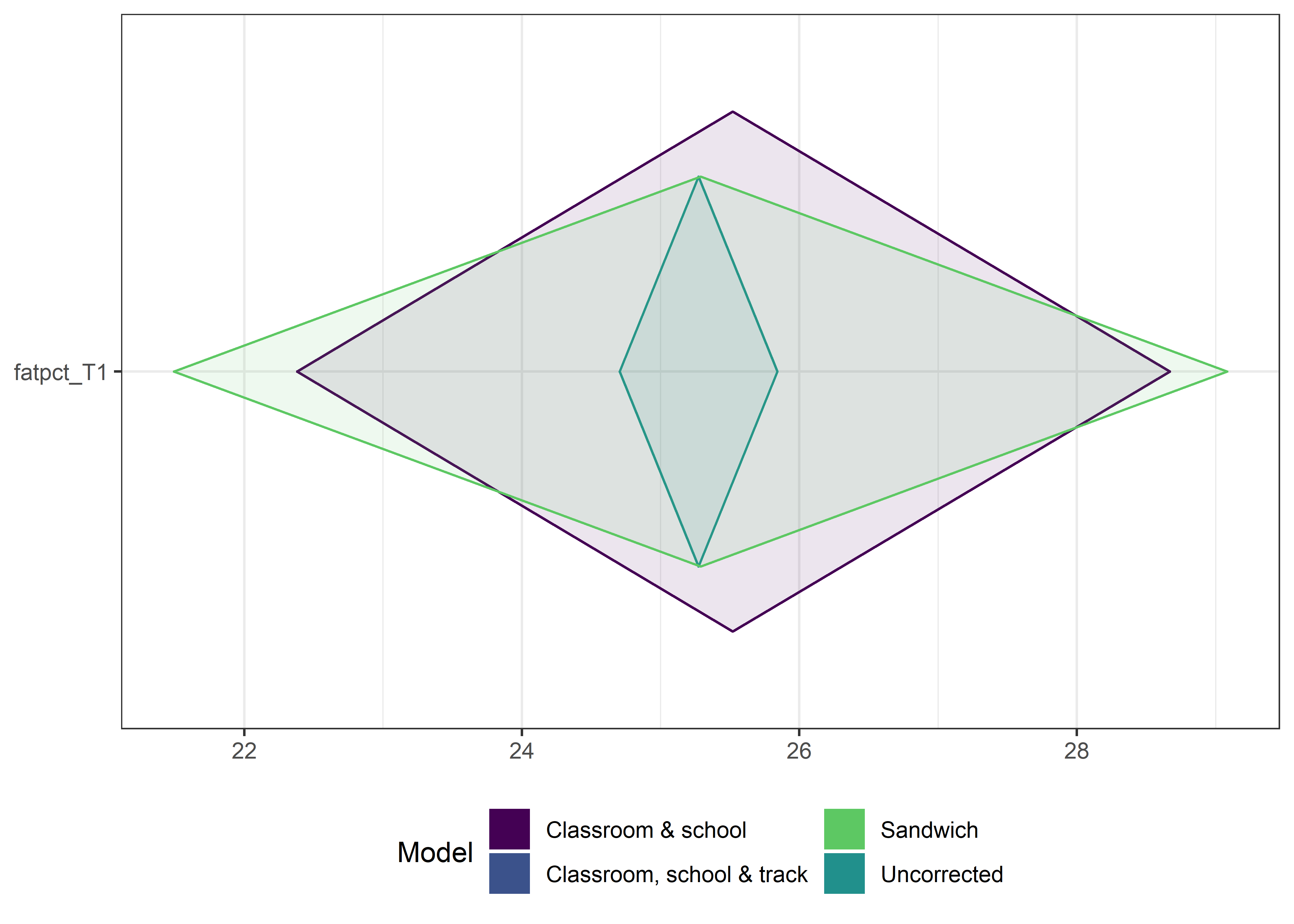
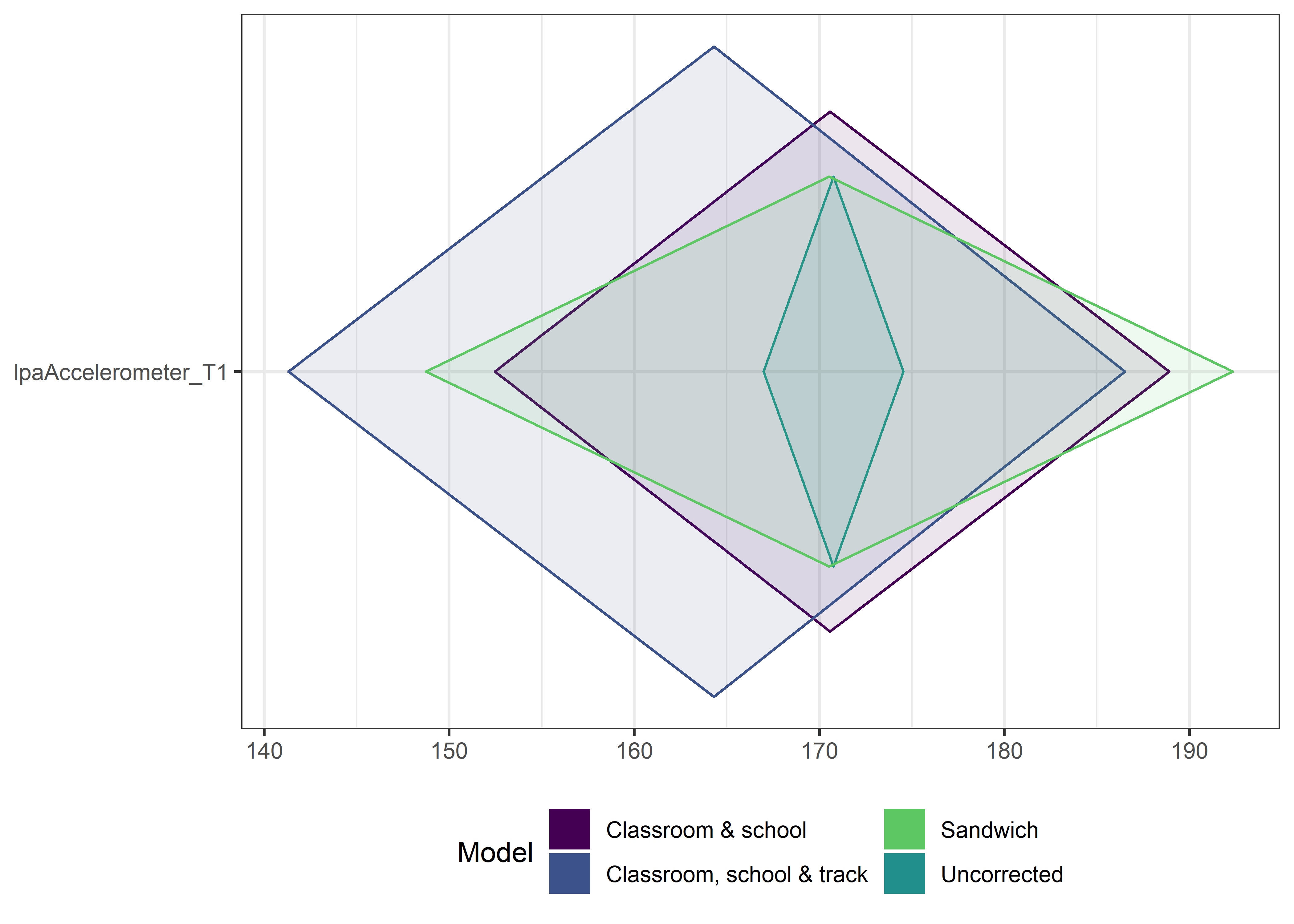
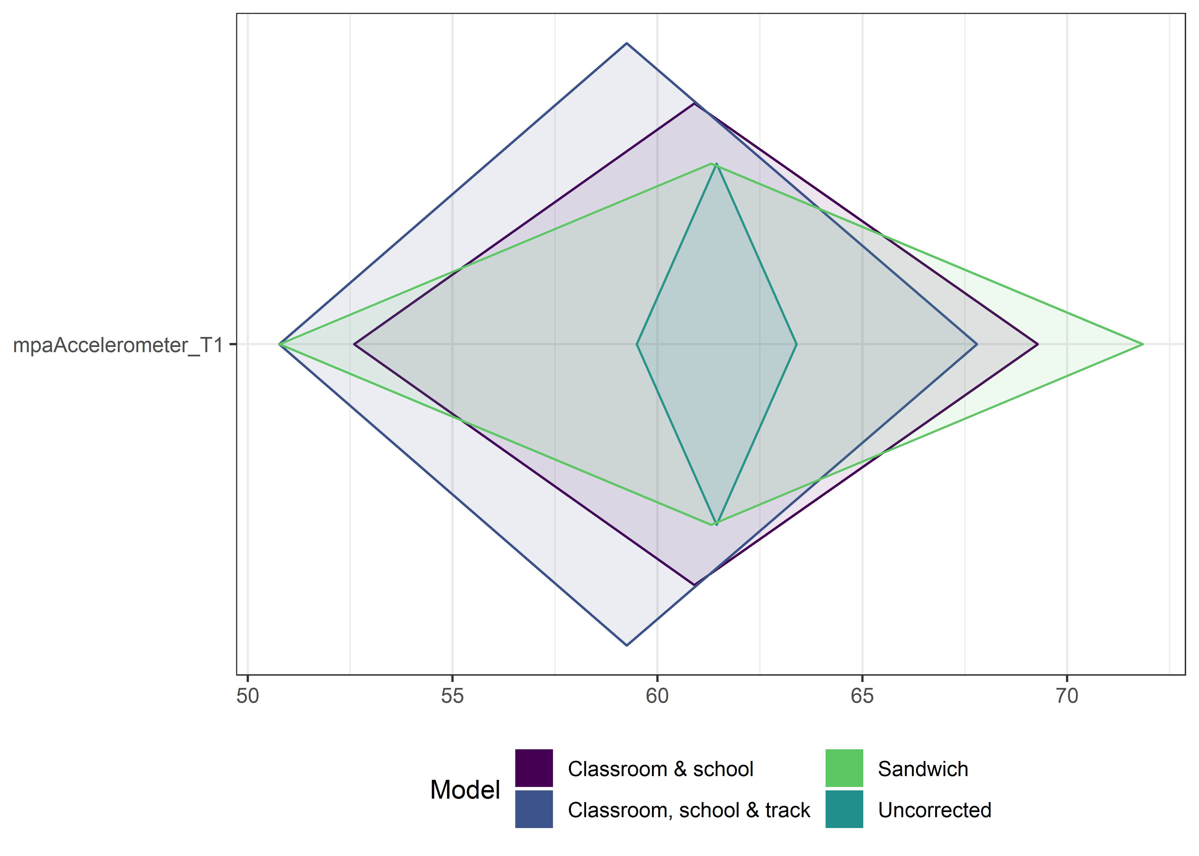
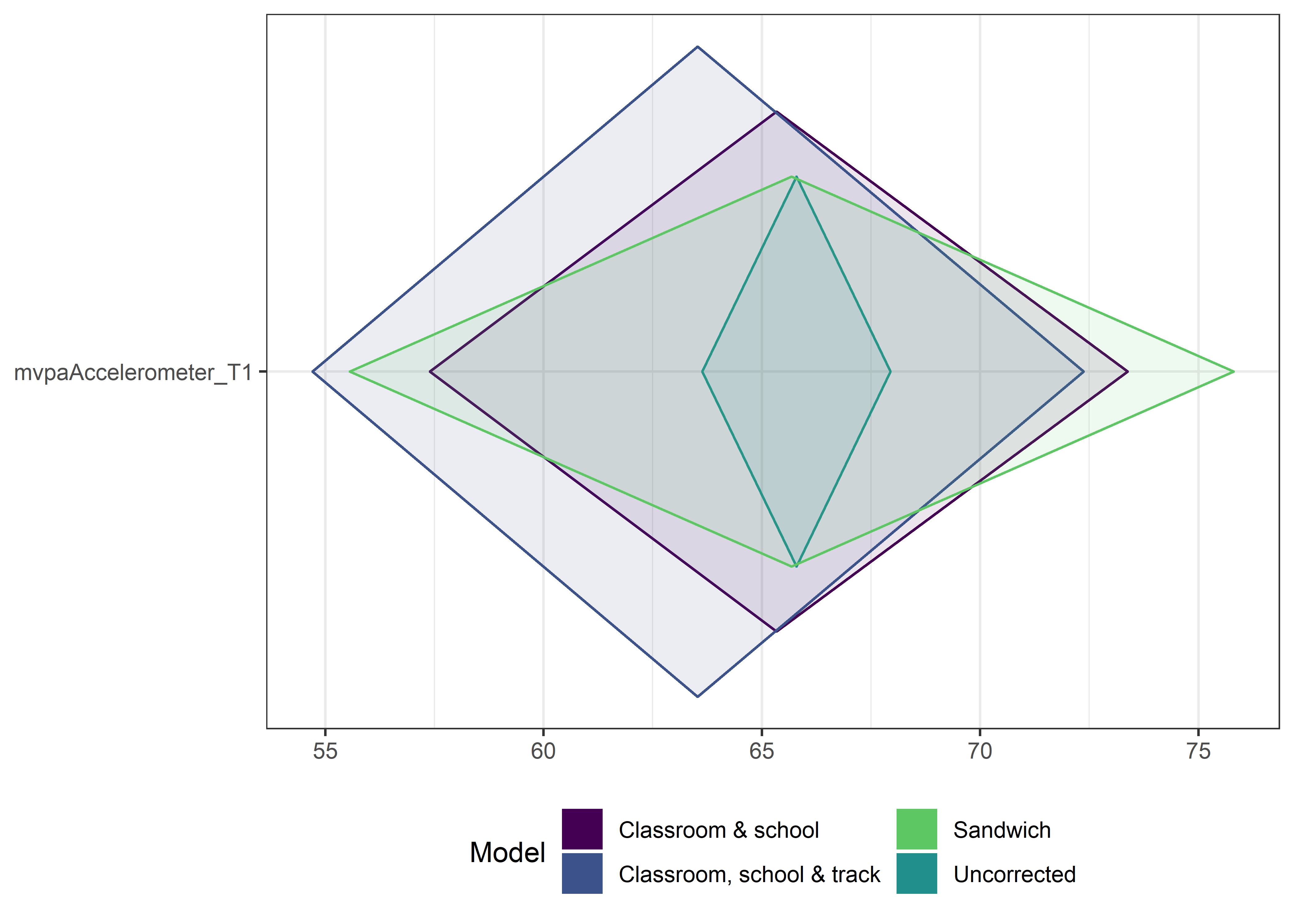
Other variables

# Take the high-mean variables out, because otherwise you'd have something with a mean of 200 
# and a mean of 2 in the same plot, and scaling of the x-axis would smudge differences between the
# diamonds, which indicate the estimates

ci_total_small <- ci_total %>% dplyr::filter(mean <= 10)
ci_edutrack_small <- ci_edutrack %>% dplyr::filter(mean <= 10)
ci_uncorrected_small <- ci_uncorrected %>% dplyr::filter(mean <= 10)
ci_sandwich_small <- ci_sandwich %>% dplyr::filter(mean <= 10)
# ci_bayes_small <- ci_bayes %>% dplyr::filter(mean <= 10)
# ci_bayes_containing_edutrack_small <- ci_bayes_containing_edutrack %>% dplyr::filter(mean <= 10)

# Now, four data frames contain columns ciLo, mean, ciHi, and variable name, for each variable (i.e. row).
# Make a diamondPlot layer from each of these data frames, so that i number of variables are in the same plot: 

for (i in c(seq(from = 1, to = nrow(ci_total_small), by = 6))) {
plot1 <- userfriendlyscience::diamondPlot(ci_total_small[i:(i + 6), ], 
                                          color = viridis::viridis(5)[1], 
                                          alpha = 0.1, 
                                          yLabels = ci_total_small[i:(i + 6), ]$diamondlabels, 
                                          fixedSize = 0.4, 
                                          xlab = NULL) +
  userfriendlyscience::diamondPlot(ci_edutrack_small[i:(i + 6), ], 
                                   returnLayerOnly = TRUE,
                                   color = viridis::viridis(5)[2], 
                                   alpha = 0.1, 
                                   yLabels = ci_edutrack_small[i:(i + 6), ]$diamondlabels, 
                                   fixedSize = 0.5, 
                                   xlab = NULL) +
  userfriendlyscience::diamondPlot(ci_uncorrected_small[i:(i + 6), ], 
                                   returnLayerOnly = TRUE,
                                   color = viridis::viridis(5)[3], 
                                   alpha = 0.1, 
                                   yLabels = ci_uncorrected_small[i:(i + 6), ]$diamondlabels, 
                                   fixedSize = 0.3, 
                                   xlab = NULL) +
  userfriendlyscience::diamondPlot(ci_sandwich_small[i:(i + 6), ], 
                                   returnLayerOnly = TRUE,
                                   color = viridis::viridis(5)[4], 
                                   alpha = 0.1, 
                                   yLabels = ci_uncorrected_small[i:(i + 6), ]$diamondlabels, 
                                   fixedSize = 0.3, 
                                   xlab = NULL) +
  # geom_point(aes(x = ci_bayes_small$ciLo[i:(i + 6)], y = 1:7),
  #            color = "red") +
  # geom_point(aes(x = ci_bayes_small$ciHi[i:(i + 6)], y = 1:7),
  #            color = "red") +
  # geom_point(aes(x = ci_bayes_containing_edutrack_small$ciLo[i:(i + 6)], y = 1:7),
  #            color = viridis::viridis(5)[5]) +
  # geom_point(aes(x = ci_bayes_containing_edutrack_small$ciHi[i:(i + 6)], y = 1:7),
  #            color = viridis::viridis(5)[5]) +
  # userfriendlyscience::diamondPlot(ci_bayes_small[i:(i + 6), ], 
  #                                  returnLayerOnly = TRUE,
  #                                  color = viridis::viridis(5)[5], 
  #                                  alpha = 0, 
  #                                  yLabels = ci_uncorrected_small[i:(i + 6), ]$diamondlabels, 
  #                                  fixedSize = 0.10, 
  #                                  xlab = NULL,
  #                                  linetype = "dashed"
  #                                  ) +
  # userfriendlyscience::diamondPlot(ci_bayes_containing_edutrack_small[i:(i + 6), ], 
  #                                  returnLayerOnly = TRUE,
  #                                  color = "red", 
  #                                  alpha = 0, 
  #                                  yLabels = ci_uncorrected_small[i:(i + 6), ]$diamondlabels, 
  #                                  fixedSize = 0.15, 
  #                                  xlab = NULL,
  #                                  linetype = "dashed"
  #                                  ) +
  geom_rect(aes(xmin=Inf, xmax=Inf, ymin=Inf, ymax=Inf, fill = "Classroom & school"), 
            colour=NA, alpha=0.05) + # Create invisible rectangle for legend
  geom_rect(aes(xmin=Inf, xmax=Inf, ymin=Inf, ymax=Inf, fill = "Classroom, school & track"), 
            colour=NA, alpha=0.05) + # Create invisible rectangle for legend
  geom_rect(aes(xmin=Inf, xmax=Inf, ymin=Inf, ymax=Inf, fill = "Uncorrected"), 
            colour=NA, alpha=0.05) + # Create invisible rectangle for legend
  geom_rect(aes(xmin=Inf, xmax=Inf, ymin=Inf, ymax=Inf, fill = "Sandwich"), 
            colour=NA, alpha=0.05) + # Create invisible rectangle for legend
  # geom_rect(aes(xmin=Inf, xmax=Inf, ymin=Inf, ymax=Inf, fill = "Bayes: classroom & school"), 
  #           colour=NA, alpha=0.05) + # Create invisible rectangle for legend
  # geom_rect(aes(xmin=Inf, xmax=Inf, ymin=Inf, ymax=Inf, fill = "Bayes: classroom, school & track"), 
  #           colour=NA, alpha=0.05) + # Create invisible rectangle for legend
  scale_fill_manual('Model: ',
                    values = c(
                      # "red",
                      #          viridis::viridis(5)[5],
                               viridis::viridis(5)[1], 
                               viridis::viridis(5)[2], 
                               viridis::viridis(5)[4], 
                               viridis::viridis(5)[3]),
                    guide = guide_legend(override.aes = list(alpha = 1), ncol = 3)) +
  theme(legend.position = "bottom", 
        legend.justification = "left",
        plot.margin = margin(t = 0, r = 4, b = 0, l = 0, unit = "cm"),
        axis.text.y = element_text(angle = 30, hjust = 1)) 
#  cat('\n\n####', i, '\n\n  ') 
  print(plot1)
}

Demographic tables

Next code chunk prepares data.


demographics <- lmi %>% dplyr::select(id = ID,
  birthYear = Kys0004.1,
  surveyDate = StartDateTime.1,
  intervention = ryhma,
  school = Aineisto.1,
  girl = Kys0013.1,
  ethnicity1 = Kys0005.1,
  ethnicity2 = Kys0005.2,
  ethnicity3 = Kys0005.3,
  studyYear = Kys0014.1) %>% 
  dplyr::mutate(
    surveyYear = lubridate::year(surveyDate),
    age = as.numeric(surveyYear) - as.numeric(birthYear),
    intervention = ifelse(intervention == 1, 1, 0),
    intervention = as.numeric(intervention, levels = c("0", "1")),
    girl = ifelse(girl == "2", 1, 0),
    girl = as.numeric(girl, levels = c("1", "0")),
    school = factor(school, levels = c("1", "2", "3", "4", "5")),
    bornInFinland = ifelse(!is.na(ethnicity1), ethnicity1, 
                           ifelse(!is.na(ethnicity2), ethnicity2,
                                  ifelse(!is.na(ethnicity3), ethnicity3, NA))),
    bornInFinland = as.numeric(ifelse(bornInFinland == 1, 1, 0)),
    studyYear = ifelse(as.numeric(studyYear) == 0, NA, as.numeric(studyYear))) %>%  # Remove "other" from study year
  dplyr::select(-surveyDate, -surveyYear, -ethnicity1, -ethnicity2, -ethnicity3)

# Insert track variable with those who answered "other" with one of the actual category labels given the appropriate category:
Track <- lmi %>% dplyr::select(Kys0016.1, Kys0017.1) %>% dplyr::mutate(
  Kys0016.1 = as.character(Kys0016.1), # Because I had an Evaluation error: `x` and `labels` must be same type.
  Kys0017.1 = as.character(Kys0017.1),
  Kys0016.1 = ifelse(Kys0017.1 == "Merkonomi" | Kys0017.1 == "merkonomi", 3,
                     ifelse(Kys0017.1 == "Datanomi" | Kys0017.1 == "datanomi", 2, Kys0016.1)),
  Track = factor(Kys0016.1, # Fix track labels first
                 levels = c(0, 1, 2, 3, 4),
                 labels = c("Other", "IT", "BA", "HRC", "Nur"))) %>% 
  dplyr::select(-Kys0016.1, -Kys0017.1)

demographics <- bind_cols(demographics, Track)

save(demographics, file = "./data/demographics.Rdata")

By educational track

demotable <- demographics %>% 
  dplyr::filter(track != "Other") %>% 
  dplyr::group_by(Track) %>% 
  dplyr::summarise(
    n = n(),
    "Mean age (range, median)" = paste0(round(mean(age, na.rm = TRUE), 1) %>% format(., nsmall = 1)," (", 
                                range(age, na.rm = TRUE)[1] %>% format(., nsmall = 1), "-",
                                range(age, na.rm = TRUE)[2] %>% format(., nsmall = 1), ", ",
                                round(median(age, na.rm = TRUE), 1) %>% format(., nsmall = 1), ")"),
    "Mean study year (sd, median)" = paste0(round(mean(studyYear, na.rm = TRUE), 1) %>% format(., nsmall = 1)," (", 
                                    round(sd(studyYear, na.rm = TRUE), 1) %>% format(., nsmall = 1), ", ",
                                    round(median(studyYear, na.rm = TRUE), 1) %>% format(., nsmall = 1), ")"),
    "% girl" = round(mean(girl, na.rm = TRUE)*100, 1) %>% format(., nsmall = 1),
    "% allocated to intervention" = round(mean(intervention, na.rm = TRUE)*100, 1) %>% format(., nsmall = 1),
    "Born in Finland (%)" = round(mean(bornInFinland, na.rm = TRUE)*100, 1) %>% format(., nsmall = 1)
                                ) %>% 
  dplyr::filter(complete.cases(.)) %>% 
  dplyr::arrange(desc(Track)) 

demotable_total <- demographics %>% 
  summarise(
    n = n(),
    "Track" = "Full sample",
    "Mean age (range, median)" = paste0(round(mean(age, na.rm = TRUE), 1) %>% format(., nsmall = 1)," (", 
                                range(age, na.rm = TRUE)[1] %>% format(., nsmall = 1), "-",
                                range(age, na.rm = TRUE)[2] %>% format(., nsmall = 1), ", ",
                                round(median(age, na.rm = TRUE), 1) %>% format(., nsmall = 1), ")"),
    "Mean study year (sd, median)" = paste0(round(mean(studyYear, na.rm = TRUE), 1) %>% format(., nsmall = 1)," (", 
                                    round(sd(studyYear, na.rm = TRUE), 1) %>% format(., nsmall = 1), ", ",
                                    round(median(studyYear, na.rm = TRUE), 1) %>% format(., nsmall = 1), ")"),
    "% girl" = round(mean(girl, na.rm = TRUE)*100, 1) %>% format(., nsmall = 1),
    "% allocated to intervention" = round(mean(intervention, na.rm = TRUE)*100, 1) %>% format(., nsmall = 1),
    "Born in Finland (%)" = round(mean(bornInFinland, na.rm = TRUE)*100, 1) %>% format(., nsmall = 1)
    )

demotable <- bind_rows(demotable, demotable_total)

demotable <- demotable %>% 
  tidyr::gather(Variable, val, 2:ncol(demotable)) %>% 
  tidyr::spread(Track, val) %>% 
  dplyr::select(Variable, Nur, HRC, BA, IT, `Full sample`) %>% 
  dplyr::arrange(-row_number())

# For some reason, sum of n's of all tracks is 1084.

save(demotable, file = "./Rdata_files/demotable.Rdata")

papaja::apa_table(demotable, caption = "Baseline demographics of educational tracks", digits = c(0, 1, 1, 1, 1, 1, 0))

(#tab:demographics-table-track) Baseline demographics of educational tracks

Variable	Nur	HRC	BA	IT	Full sample	NA
n	402	213	282	163	1166	n
Mean study year (sd, median)	1.7 (0.9, 1.0)	1.9 (0.7, 2.0)	1.7 (0.9, 1.0)	1.7 (0.9, 1.0)	1.7 (0.9, 1.0)	Mean study year (sd, median)
Mean age (range, median)	18.8 (16.0-49.0, 17.0)	18.5 (17.0-27.0, 18.0)	18.0 (16.0-35.0, 17.0)	18.5 (17.0-43.0, 17.0)	18.5 (16.0-49.0, 18.0)	Mean age (range, median)
Born in Finland (%)	80.1	88.3	89.7	86.7	84.4	Born in Finland (%)
% girl	82.3	60.6	39.0	16.0	56.5	% girl
% allocated to intervention	68.9	31.5	53.5	46.6	54.7	% allocated to intervention

By gender

# demographics$Girl <- factor(demographics$girl)

demotable <- demographics %>% 
  group_by(girl) %>% 
  summarise(
    n = n(),
    "Mean age (range, median)" = paste0(round(mean(age, na.rm = TRUE), 1) %>% format(., nsmall = 1)," (", 
                                range(age, na.rm = TRUE)[1] %>% format(., nsmall = 1), "-",
                                range(age, na.rm = TRUE)[2] %>% format(., nsmall = 1), ", ",
                                round(median(age, na.rm = TRUE), 1) %>% format(., nsmall = 1), ")"),
    "Mean study year (sd, median)" = paste0(round(mean(studyYear, na.rm = TRUE), 1) %>% format(., nsmall = 1)," (", 
                                    round(sd(studyYear, na.rm = TRUE), 1) %>% format(., nsmall = 1), ", ",
                                    round(median(studyYear, na.rm = TRUE), 1) %>% format(., nsmall = 1), ")"),
    "% allocated to intervention" = round(mean(intervention, na.rm = TRUE)*100, 1) %>% format(., nsmall = 1),
    "Born in Finland (%)" = round(mean(bornInFinland, na.rm = TRUE)*100, 1) %>% format(., nsmall = 1)
    ) %>% 
  dplyr::filter(complete.cases(.)) %>% 
  arrange(desc(girl)) 

demotable_total <- demographics %>% 
  summarise(
    n = n(),
    "Mean age (range, median)" = paste0(round(mean(age, na.rm = TRUE), 1) %>% format(., nsmall = 1)," (", 
                                range(age, na.rm = TRUE)[1] %>% format(., nsmall = 1), "-",
                                range(age, na.rm = TRUE)[2] %>% format(., nsmall = 1), ", ",
                                round(median(age, na.rm = TRUE), 1) %>% format(., nsmall = 1), ")"),
    "Mean study year (sd, median)" = paste0(round(mean(studyYear, na.rm = TRUE), 1) %>% format(., nsmall = 1)," (", 
                                    round(sd(studyYear, na.rm = TRUE), 1) %>% format(., nsmall = 1), ", ",
                                    round(median(studyYear, na.rm = TRUE), 1) %>% format(., nsmall = 1), ")"),
    "% allocated to intervention" = round(mean(intervention, na.rm = TRUE)*100, 1) %>% format(., nsmall = 1),
    "Born in Finland (%)" = round(mean(bornInFinland, na.rm = TRUE)*100, 1) %>% format(., nsmall = 1)
    )

demotable <- bind_rows(demotable, demotable_total)

demotable <- demotable %>% 
  tidyr::gather(Variable, val, 2:ncol(demotable)) %>% 
  tidyr::spread(girl, val) %>% 
  dplyr::arrange(-row_number())

names(demotable) <- c("", "Boy", "Girl", "Full sample")

# For some reason, sum of n's of all tracks is 1084.

papaja::apa_table(demotable, caption = "Baseline demographics of educational tracks", digits = c(0, 1, 1, 1, 1, 0))

(#tab:demographics-table-gender) Baseline demographics of educational tracks

	Boy	Girl	Full sample	NA	NA
n	471	613	1166	n	471
Mean study year (sd, median)	1.7 (0.9, 1.0)	1.7 (0.8, 1.0)	1.7 (0.9, 1.0)	Mean study year (sd, median)	1.7 (0.9, 1.0)
Mean age (range, median)	18.2 (16.0-35.0, 18.0)	18.7 (16.0-49.0, 18.0)	18.5 (16.0-49.0, 18.0)	Mean age (range, median)	18.2 (16.0-35.0, 18.0)
Born in Finland (%)	89.1	80.7	84.4	Born in Finland (%)	89.1
% allocated to intervention	50.5	56.0	54.7	% allocated to intervention	50.5

By intervention participation

demographics$intervention <- factor(demographics$intervention)
demographics$girl <- as.numeric(demographics$girl)

demotable <- demographics %>% 
  group_by(intervention) %>% 
  summarise(
    "Mean age (range, median)" = paste0(round(mean(age, na.rm = TRUE), 1) %>% format(., nsmall = 1)," (", 
                                range(age, na.rm = TRUE)[1] %>% format(., nsmall = 1), "-",
                                range(age, na.rm = TRUE)[2] %>% format(., nsmall = 1), ", ",
                                round(median(age, na.rm = TRUE), 1) %>% format(., nsmall = 1), ")"),
    "Mean study year (sd, median)" = paste0(round(mean(studyYear, na.rm = TRUE), 1) %>% format(., nsmall = 1)," (", 
                                    round(sd(studyYear, na.rm = TRUE), 1) %>% format(., nsmall = 1), ", ",
                                    round(median(studyYear, na.rm = TRUE), 1) %>% format(., nsmall = 1), ")"),
    "% girl" = round(mean(girl, na.rm = TRUE)*100, 1) %>% format(., nsmall = 1),
    "Born in Finland (%)" = round(mean(bornInFinland, na.rm = TRUE)*100, 1) %>% format(., nsmall = 1),
    n = n()
    ) %>% 
  dplyr::filter(complete.cases(.)) %>% 
  arrange(desc(intervention)) 

demotable_total <- demographics %>% 
  summarise(
    "intervention" = "Full sample",
    "Mean age (range, median)" = paste0(round(mean(age, na.rm = TRUE), 1) %>% format(., nsmall = 1)," (", 
                                range(age, na.rm = TRUE)[1] %>% format(., nsmall = 1), "-",
                                range(age, na.rm = TRUE)[2] %>% format(., nsmall = 1), ", ",
                                round(median(age, na.rm = TRUE), 1) %>% format(., nsmall = 1), ")"),
    "Mean study year (sd, median)" = paste0(round(mean(studyYear, na.rm = TRUE), 1) %>% format(., nsmall = 1)," (", 
                                    round(sd(studyYear, na.rm = TRUE), 1) %>% format(., nsmall = 1), ", ",
                                    round(median(studyYear, na.rm = TRUE), 1) %>% format(., nsmall = 1), ")"),
    "% girl" = round(mean(girl, na.rm = TRUE)*100, 1) %>% format(., nsmall = 1),
    "Born in Finland (%)" = round(mean(bornInFinland, na.rm = TRUE)*100, 1) %>% format(., nsmall = 1),
    n = n()
    )

demotable <- bind_rows(demotable, demotable_total)

demotable <- demotable %>% 
  tidyr::gather(Variable, val, 2:ncol(demotable)) %>% 
  tidyr::spread(intervention, val) %>% 
  dplyr::arrange(-row_number())

names(demotable) <- c("", "Control", "Intervention", "Full sample")

# For some reason, sum of n's of all tracks is 1084.

papaja::apa_table(demotable, caption = "Baseline demographics of educational tracks", digits = c(0, 1, 1, 1, 1, 0))

(#tab:demographics-table-intervention) Baseline demographics of educational tracks

	Control	Intervention	Full sample	NA	NA
n	528	638	1166	n	528
Mean study year (sd, median)	1.7 (0.9, 1.0)	1.7 (0.9, 1.0)	1.7 (0.9, 1.0)	Mean study year (sd, median)	1.7 (0.9, 1.0)
Mean age (range, median)	18.3 (16.0-38.0, 17.0)	18.7 (16.0-49.0, 18.0)	18.5 (16.0-49.0, 18.0)	Mean age (range, median)	18.3 (16.0-38.0, 17.0)
Born in Finland (%)	88.7	80.5	84.4	Born in Finland (%)	88.7
% girl	53.7	59.0	56.5	% girl	53.7

Outcome tables


outtable_track <- df %>%
  dplyr::select(mvpaAccelerometer_T1, sitLieAccelerometer_T1, sitBreaksAccelerometer_T1, # Main outcomes 
          weartimeAccelerometer_T1,
          PA_actionplan_T1,
          PA_copingplan_T1,
          PA_agreementDependentBCT_T1,
          PA_frequencyDependentBCT_T1,
          PA_amotivation_T1,
          PA_autonomous_T1,
          PA_controlled_T1,
          PA_goal_T1,
          PA_injunctiveNorm_T1,
          PA_descriptiveNorm_T1,
          PA_intention_T1,
          PA_outcomeExpectations_T1,
          PA_opportunities_T1,
          PA_perceivedBehaviouralControl_T1,
          PA_selfefficacy_T1,
          SB_descriptiveNorm_T1,
          SB_injunctiveNorm_T1,
          SB_intention_T1,
          SB_outcomeExpectations_T1,
          SB_selfEfficacyperceivedBehaviouralControl_T1,
         track, girl, intervention) %>% 
  group_by(track) %>% 
  summarise(
            "PA action planning" = paste0(round(mean(PA_actionplan_T1, na.rm = TRUE), 1) %>% format(., nsmall = 1), 
                                          " (", round(sd(PA_actionplan_T1, na.rm = TRUE), 1) %>% format(., nsmall = 1), ")"),
            "PA coping planning" = paste0(round(mean(PA_copingplan_T1, na.rm = TRUE), 1) %>% format(., nsmall = 1), 
                                          " (", round(sd(PA_copingplan_T1, na.rm = TRUE), 1) %>% format(., nsmall = 1), ")"),
            "PA agreement-BCTs" = paste0(round(mean(PA_agreementDependentBCT_T1, na.rm = TRUE), 1) %>% format(., nsmall = 1), 
                                         " (", round(sd(PA_agreementDependentBCT_T1, na.rm = TRUE), 1) %>% format(., nsmall = 1), ")"),
            "PA frequency-BCTs" = paste0(round(mean(PA_frequencyDependentBCT_T1, na.rm = TRUE), 1) %>% format(., nsmall = 1), 
                                         " (", round(sd(PA_frequencyDependentBCT_T1, na.rm = TRUE), 1) %>% format(., nsmall = 1), ")"),
            "PA amotivation" = paste0(round(mean(PA_amotivation_T1, na.rm = TRUE), 1) %>% format(., nsmall = 1), 
                                      " (", round(sd(PA_amotivation_T1, na.rm = TRUE), 1) %>% format(., nsmall = 1), ")"),
            "PA autonomous regulation" = paste0(round(mean(PA_autonomous_T1, na.rm = TRUE), 1) %>% format(., nsmall = 1), 
                                                " (", round(sd(PA_autonomous_T1, na.rm = TRUE), 1) %>% format(., nsmall = 1), ")"),
            "PA controlled regulation" = paste0(round(mean(PA_controlled_T1, na.rm = TRUE), 1) %>% format(., nsmall = 1), 
                                                " (", round(sd(PA_controlled_T1, na.rm = TRUE), 1) %>% format(., nsmall = 1), ")"),
            "PA injunctive norm" = paste0(round(mean(PA_injunctiveNorm_T1, na.rm = TRUE), 1) %>% format(., nsmall = 1), 
                                          " (", round(sd(PA_injunctiveNorm_T1, na.rm = TRUE), 1) %>% format(., nsmall = 1), ")"),
            "PA descriptive norm" = paste0(round(mean(PA_descriptiveNorm_T1, na.rm = TRUE), 1) %>% format(., nsmall = 1), 
                                           " (", round(sd(PA_descriptiveNorm_T1, na.rm = TRUE), 1) %>% format(., nsmall = 1), ")"),
            "PA intention" = paste0(round(mean(PA_intention_T1, na.rm = TRUE), 1) %>% format(., nsmall = 1), 
                                    " (", round(sd(PA_intention_T1, na.rm = TRUE), 1) %>% format(., nsmall = 1), ")"),
            "PA outcome expectations" = paste0(round(mean(PA_outcomeExpectations_T1, na.rm = TRUE), 1) %>% format(., nsmall = 1), 
                                               " (", round(sd(PA_outcomeExpectations_T1, na.rm = TRUE), 1) %>% format(., nsmall = 1), ")"),
            "PA opportunities" = paste0(round(mean(PA_opportunities_T1, na.rm = TRUE), 1) %>% format(., nsmall = 1), 
                                        " (", round(sd(PA_opportunities_T1, na.rm = TRUE), 1) %>% format(., nsmall = 1), ")"),
            "PA perceived behavioural control" = paste0(round(mean(PA_perceivedBehaviouralControl_T1, na.rm = TRUE), 1) %>% format(., nsmall = 1), 
                                                        " (", round(sd(PA_perceivedBehaviouralControl_T1, na.rm = TRUE), 1) %>% format(., nsmall = 1), ")"),
            "PA self-efficacy" = paste0(round(mean(PA_selfefficacy_T1, na.rm = TRUE), 1) %>% format(., nsmall = 1), 
                                        " (", round(sd(PA_selfefficacy_T1, na.rm = TRUE), 1) %>% format(., nsmall = 1), ")"),
            "SB descriptive norm" = paste0(round(mean(SB_descriptiveNorm_T1, na.rm = TRUE), 1) %>% format(., nsmall = 1), 
                                           " (", round(sd(SB_descriptiveNorm_T1, na.rm = TRUE), 1) %>% format(., nsmall = 1), ")"),
            "SB injunctive norm" = paste0(round(mean(SB_injunctiveNorm_T1, na.rm = TRUE), 1) %>% format(., nsmall = 1), 
                                          " (", round(sd(SB_injunctiveNorm_T1, na.rm = TRUE), 1) %>% format(., nsmall = 1), ")"),
            "SB intention" = paste0(round(mean(SB_intention_T1, na.rm = TRUE), 1) %>% format(., nsmall = 1), 
                                    " (", round(sd(SB_intention_T1, na.rm = TRUE), 1) %>% format(., nsmall = 1), ")"),
            "SB outcome expectations" = paste0(round(mean(SB_outcomeExpectations_T1, na.rm = TRUE), 1) %>% format(., nsmall = 1), 
                                               " (", round(sd(SB_outcomeExpectations_T1, na.rm = TRUE), 1) %>% format(., nsmall = 1), ")"),
            "SB self-efficacy & perceived behavioural control" = paste0(round(mean(SB_selfEfficacyperceivedBehaviouralControl_T1, na.rm = TRUE), 1) %>% format(., nsmall = 1), 
                                                                        " (", round(sd(SB_selfEfficacyperceivedBehaviouralControl_T1, na.rm = TRUE), 1) %>% format(., nsmall = 1), ")"),
            "Mean daily MVPA hours" = paste0(round(mean(mvpaAccelerometer_T1, na.rm = TRUE), 1) %>% format(., nsmall = 1),
                                               " (", round(sd(mvpaAccelerometer_T1, na.rm = TRUE), 1) %>% format(., nsmall = 1), ")"),
            "Mean daily hours spent sitting or lying down" = paste0(round(mean(sitLieAccelerometer_T1, na.rm = TRUE), 1) %>% format(., nsmall = 1),
                                                                      " (", round(sd(sitLieAccelerometer_T1, na.rm = TRUE), 1) %>% format(., nsmall = 1), ")"),
            "Mean daily breaks in sitting" = paste0(round(mean(sitBreaksAccelerometer_T1, na.rm = TRUE), 1) %>% format(., nsmall = 1),
                                                    " (", round(sd(sitBreaksAccelerometer_T1, na.rm = TRUE), 1) %>% format(., nsmall = 1), ")"),
            "Mean daily accelerometer weartime hours" = paste0(round(mean(weartimeAccelerometer_T1, na.rm = TRUE), 1) %>% format(., nsmall = 1),
                                                    " (", round(sd(weartimeAccelerometer_T1, na.rm = TRUE), 1) %>% format(., nsmall = 1), ")"),
            n = n()) %>% 
  dplyr::filter(complete.cases(.)) %>% 
  arrange((track)) %>% 
  dplyr::filter(track != "Other")

outtable_intervention <- df %>%
  dplyr::select(mvpaAccelerometer_T1, sitLieAccelerometer_T1, sitBreaksAccelerometer_T1, # Main outcomes  
          weartimeAccelerometer_T1,
          PA_actionplan_T1,
          PA_copingplan_T1,
          PA_agreementDependentBCT_T1,
          PA_frequencyDependentBCT_T1,
          PA_amotivation_T1,
          PA_autonomous_T1,
          PA_controlled_T1,
          PA_goal_T1,
          PA_injunctiveNorm_T1,
          PA_descriptiveNorm_T1,
          PA_intention_T1,
          PA_outcomeExpectations_T1,
          PA_opportunities_T1,
          PA_perceivedBehaviouralControl_T1,
          PA_selfefficacy_T1,
          SB_descriptiveNorm_T1,
          SB_injunctiveNorm_T1,
          SB_intention_T1,
          SB_outcomeExpectations_T1,
          SB_selfEfficacyperceivedBehaviouralControl_T1,
         track, girl, intervention) %>% 
  group_by(intervention) %>% 
  summarise(
            "PA action planning" = paste0(round(mean(PA_actionplan_T1, na.rm = TRUE), 1) %>% format(., nsmall = 1), 
                                          " (", round(sd(PA_actionplan_T1, na.rm = TRUE), 1) %>% format(., nsmall = 1), ")"),
            "PA coping planning" = paste0(round(mean(PA_copingplan_T1, na.rm = TRUE), 1) %>% format(., nsmall = 1), 
                                          " (", round(sd(PA_copingplan_T1, na.rm = TRUE), 1) %>% format(., nsmall = 1), ")"),
            "PA agreement-BCTs" = paste0(round(mean(PA_agreementDependentBCT_T1, na.rm = TRUE), 1) %>% format(., nsmall = 1), 
                                         " (", round(sd(PA_agreementDependentBCT_T1, na.rm = TRUE), 1) %>% format(., nsmall = 1), ")"),
            "PA frequency-BCTs" = paste0(round(mean(PA_frequencyDependentBCT_T1, na.rm = TRUE), 1) %>% format(., nsmall = 1), 
                                         " (", round(sd(PA_frequencyDependentBCT_T1, na.rm = TRUE), 1) %>% format(., nsmall = 1), ")"),
            "PA amotivation" = paste0(round(mean(PA_amotivation_T1, na.rm = TRUE), 1) %>% format(., nsmall = 1), 
                                      " (", round(sd(PA_amotivation_T1, na.rm = TRUE), 1) %>% format(., nsmall = 1), ")"),
            "PA autonomous regulation" = paste0(round(mean(PA_autonomous_T1, na.rm = TRUE), 1) %>% format(., nsmall = 1), 
                                                " (", round(sd(PA_autonomous_T1, na.rm = TRUE), 1) %>% format(., nsmall = 1), ")"),
            "PA controlled regulation" = paste0(round(mean(PA_controlled_T1, na.rm = TRUE), 1) %>% format(., nsmall = 1), 
                                                " (", round(sd(PA_controlled_T1, na.rm = TRUE), 1) %>% format(., nsmall = 1), ")"),
            "PA injunctive norm" = paste0(round(mean(PA_injunctiveNorm_T1, na.rm = TRUE), 1) %>% format(., nsmall = 1), 
                                          " (", round(sd(PA_injunctiveNorm_T1, na.rm = TRUE), 1) %>% format(., nsmall = 1), ")"),
            "PA descriptive norm" = paste0(round(mean(PA_descriptiveNorm_T1, na.rm = TRUE), 1) %>% format(., nsmall = 1), 
                                           " (", round(sd(PA_descriptiveNorm_T1, na.rm = TRUE), 1) %>% format(., nsmall = 1), ")"),
            "PA intention" = paste0(round(mean(PA_intention_T1, na.rm = TRUE), 1) %>% format(., nsmall = 1), 
                                    " (", round(sd(PA_intention_T1, na.rm = TRUE), 1) %>% format(., nsmall = 1), ")"),
            "PA outcome expectations" = paste0(round(mean(PA_outcomeExpectations_T1, na.rm = TRUE), 1) %>% format(., nsmall = 1), 
                                               " (", round(sd(PA_outcomeExpectations_T1, na.rm = TRUE), 1) %>% format(., nsmall = 1), ")"),
            "PA opportunities" = paste0(round(mean(PA_opportunities_T1, na.rm = TRUE), 1) %>% format(., nsmall = 1), 
                                        " (", round(sd(PA_opportunities_T1, na.rm = TRUE), 1) %>% format(., nsmall = 1), ")"),
            "PA perceived behavioural control" = paste0(round(mean(PA_perceivedBehaviouralControl_T1, na.rm = TRUE), 1) %>% format(., nsmall = 1), 
                                                        " (", round(sd(PA_perceivedBehaviouralControl_T1, na.rm = TRUE), 1) %>% format(., nsmall = 1), ")"),
            "PA self-efficacy" = paste0(round(mean(PA_selfefficacy_T1, na.rm = TRUE), 1) %>% format(., nsmall = 1), 
                                        " (", round(sd(PA_selfefficacy_T1, na.rm = TRUE), 1) %>% format(., nsmall = 1), ")"),
            "SB descriptive norm" = paste0(round(mean(SB_descriptiveNorm_T1, na.rm = TRUE), 1) %>% format(., nsmall = 1), 
                                           " (", round(sd(SB_descriptiveNorm_T1, na.rm = TRUE), 1) %>% format(., nsmall = 1), ")"),
            "SB injunctive norm" = paste0(round(mean(SB_injunctiveNorm_T1, na.rm = TRUE), 1) %>% format(., nsmall = 1), 
                                          " (", round(sd(SB_injunctiveNorm_T1, na.rm = TRUE), 1) %>% format(., nsmall = 1), ")"),
            "SB intention" = paste0(round(mean(SB_intention_T1, na.rm = TRUE), 1) %>% format(., nsmall = 1), 
                                    " (", round(sd(SB_intention_T1, na.rm = TRUE), 1) %>% format(., nsmall = 1), ")"),
            "SB outcome expectations" = paste0(round(mean(SB_outcomeExpectations_T1, na.rm = TRUE), 1) %>% format(., nsmall = 1), 
                                               " (", round(sd(SB_outcomeExpectations_T1, na.rm = TRUE), 1) %>% format(., nsmall = 1), ")"),
            "SB self-efficacy & perceived behavioural control" = paste0(round(mean(SB_selfEfficacyperceivedBehaviouralControl_T1, na.rm = TRUE), 1) %>% format(., nsmall = 1), 
                                                                        " (", round(sd(SB_selfEfficacyperceivedBehaviouralControl_T1, na.rm = TRUE), 1) %>% format(., nsmall = 1), ")"),
            "Mean daily MVPA minutes" = paste0(round(mean(mvpaAccelerometer_T1, na.rm = TRUE), 1) %>% format(., nsmall = 1),
                                               " (", round(sd(mvpaAccelerometer_T1, na.rm = TRUE), 1) %>% format(., nsmall = 1), ")"),
            "Mean daily minutes spent sitting or lying down" = paste0(round(mean(sitLieAccelerometer_T1, na.rm = TRUE), 1) %>% format(., nsmall = 1),
                                                                      " (", round(sd(sitLieAccelerometer_T1, na.rm = TRUE), 1) %>% format(., nsmall = 1), ")"),
            "Mean daily breaks in sitting" = paste0(round(mean(sitBreaksAccelerometer_T1, na.rm = TRUE), 1) %>% format(., nsmall = 1),
                                                    " (", round(sd(sitBreaksAccelerometer_T1, na.rm = TRUE), 1) %>% format(., nsmall = 1), ")"),
            "Mean daily accelerometer weartime" = paste0(round(mean(weartimeAccelerometer_T1, na.rm = TRUE), 1) %>% format(., nsmall = 1),
                                                    " (", round(sd(weartimeAccelerometer_T1, na.rm = TRUE), 1) %>% format(., nsmall = 1), ")"),
            n = n()) %>% 
  dplyr::filter(complete.cases(.))

outtable_girl <- df %>%
  dplyr::select(mvpaAccelerometer_T1, sitLieAccelerometer_T1, sitBreaksAccelerometer_T1, # Main outcomes  
          weartimeAccelerometer_T1,
          PA_actionplan_T1,
          PA_copingplan_T1,
          PA_agreementDependentBCT_T1,
          PA_frequencyDependentBCT_T1,
          PA_amotivation_T1,
          PA_autonomous_T1,
          PA_controlled_T1,
          PA_goal_T1,
          PA_injunctiveNorm_T1,
          PA_descriptiveNorm_T1,
          PA_intention_T1,
          PA_outcomeExpectations_T1,
          PA_opportunities_T1,
          PA_perceivedBehaviouralControl_T1,
          PA_selfefficacy_T1,
          SB_descriptiveNorm_T1,
          SB_injunctiveNorm_T1,
          SB_intention_T1,
          SB_outcomeExpectations_T1,
          SB_selfEfficacyperceivedBehaviouralControl_T1,
         track, girl, intervention) %>% 
  group_by(girl) %>% 
  summarise(
            "PA action planning" = paste0(round(mean(PA_actionplan_T1, na.rm = TRUE), 1) %>% format(., nsmall = 1), 
                                          " (", round(sd(PA_actionplan_T1, na.rm = TRUE), 1) %>% format(., nsmall = 1), ")"),
            "PA coping planning" = paste0(round(mean(PA_copingplan_T1, na.rm = TRUE), 1) %>% format(., nsmall = 1), 
                                          " (", round(sd(PA_copingplan_T1, na.rm = TRUE), 1) %>% format(., nsmall = 1), ")"),
            "PA agreement-BCTs" = paste0(round(mean(PA_agreementDependentBCT_T1, na.rm = TRUE), 1) %>% format(., nsmall = 1), 
                                         " (", round(sd(PA_agreementDependentBCT_T1, na.rm = TRUE), 1) %>% format(., nsmall = 1), ")"),
            "PA frequency-BCTs" = paste0(round(mean(PA_frequencyDependentBCT_T1, na.rm = TRUE), 1) %>% format(., nsmall = 1), 
                                         " (", round(sd(PA_frequencyDependentBCT_T1, na.rm = TRUE), 1) %>% format(., nsmall = 1), ")"),
            "PA amotivation" = paste0(round(mean(PA_amotivation_T1, na.rm = TRUE), 1) %>% format(., nsmall = 1), 
                                      " (", round(sd(PA_amotivation_T1, na.rm = TRUE), 1) %>% format(., nsmall = 1), ")"),
            "PA autonomous regulation" = paste0(round(mean(PA_autonomous_T1, na.rm = TRUE), 1) %>% format(., nsmall = 1), 
                                                " (", round(sd(PA_autonomous_T1, na.rm = TRUE), 1) %>% format(., nsmall = 1), ")"),
            "PA controlled regulation" = paste0(round(mean(PA_controlled_T1, na.rm = TRUE), 1) %>% format(., nsmall = 1), 
                                                " (", round(sd(PA_controlled_T1, na.rm = TRUE), 1) %>% format(., nsmall = 1), ")"),
            "PA injunctive norm" = paste0(round(mean(PA_injunctiveNorm_T1, na.rm = TRUE), 1) %>% format(., nsmall = 1), 
                                          " (", round(sd(PA_injunctiveNorm_T1, na.rm = TRUE), 1) %>% format(., nsmall = 1), ")"),
            "PA descriptive norm" = paste0(round(mean(PA_descriptiveNorm_T1, na.rm = TRUE), 1) %>% format(., nsmall = 1), 
                                           " (", round(sd(PA_descriptiveNorm_T1, na.rm = TRUE), 1) %>% format(., nsmall = 1), ")"),
            "PA intention" = paste0(round(mean(PA_intention_T1, na.rm = TRUE), 1) %>% format(., nsmall = 1), 
                                    " (", round(sd(PA_intention_T1, na.rm = TRUE), 1) %>% format(., nsmall = 1), ")"),
            "PA outcome expectations" = paste0(round(mean(PA_outcomeExpectations_T1, na.rm = TRUE), 1) %>% format(., nsmall = 1), 
                                               " (", round(sd(PA_outcomeExpectations_T1, na.rm = TRUE), 1) %>% format(., nsmall = 1), ")"),
            "PA opportunities" = paste0(round(mean(PA_opportunities_T1, na.rm = TRUE), 1) %>% format(., nsmall = 1), 
                                        " (", round(sd(PA_opportunities_T1, na.rm = TRUE), 1) %>% format(., nsmall = 1), ")"),
            "PA perceived behavioural control" = paste0(round(mean(PA_perceivedBehaviouralControl_T1, na.rm = TRUE), 1) %>% format(., nsmall = 1), 
                                                        " (", round(sd(PA_perceivedBehaviouralControl_T1, na.rm = TRUE), 1) %>% format(., nsmall = 1), ")"),
            "PA self-efficacy" = paste0(round(mean(PA_selfefficacy_T1, na.rm = TRUE), 1) %>% format(., nsmall = 1), 
                                        " (", round(sd(PA_selfefficacy_T1, na.rm = TRUE), 1) %>% format(., nsmall = 1), ")"),
            "SB descriptive norm" = paste0(round(mean(SB_descriptiveNorm_T1, na.rm = TRUE), 1) %>% format(., nsmall = 1), 
                                           " (", round(sd(SB_descriptiveNorm_T1, na.rm = TRUE), 1) %>% format(., nsmall = 1), ")"),
            "SB injunctive norm" = paste0(round(mean(SB_injunctiveNorm_T1, na.rm = TRUE), 1) %>% format(., nsmall = 1), 
                                          " (", round(sd(SB_injunctiveNorm_T1, na.rm = TRUE), 1) %>% format(., nsmall = 1), ")"),
            "SB intention" = paste0(round(mean(SB_intention_T1, na.rm = TRUE), 1) %>% format(., nsmall = 1), 
                                    " (", round(sd(SB_intention_T1, na.rm = TRUE), 1) %>% format(., nsmall = 1), ")"),
            "SB outcome expectations" = paste0(round(mean(SB_outcomeExpectations_T1, na.rm = TRUE), 1) %>% format(., nsmall = 1), 
                                               " (", round(sd(SB_outcomeExpectations_T1, na.rm = TRUE), 1) %>% format(., nsmall = 1), ")"),
            "SB self-efficacy & perceived behavioural control" = paste0(round(mean(SB_selfEfficacyperceivedBehaviouralControl_T1, na.rm = TRUE), 1) %>% format(., nsmall = 1), 
                                                                        " (", round(sd(SB_selfEfficacyperceivedBehaviouralControl_T1, na.rm = TRUE), 1) %>% format(., nsmall = 1), ")"),
            "Mean daily MVPA minutes" = paste0(round(mean(mvpaAccelerometer_T1, na.rm = TRUE), 1) %>% format(., nsmall = 1),
                                               " (", round(sd(mvpaAccelerometer_T1, na.rm = TRUE), 1) %>% format(., nsmall = 1), ")"),
            "Mean daily minutes spent sitting or lying down" = paste0(round(mean(sitLieAccelerometer_T1, na.rm = TRUE), 1) %>% format(., nsmall = 1),
                                                                      " (", round(sd(sitLieAccelerometer_T1, na.rm = TRUE), 1) %>% format(., nsmall = 1), ")"),
            "Mean daily breaks in sitting" = paste0(round(mean(sitBreaksAccelerometer_T1, na.rm = TRUE), 1) %>% format(., nsmall = 1),
                                                    " (", round(sd(sitBreaksAccelerometer_T1, na.rm = TRUE), 1) %>% format(., nsmall = 1), ")"),
            "Mean daily accelerometer weartime" = paste0(round(mean(weartimeAccelerometer_T1, na.rm = TRUE), 1) %>% format(., nsmall = 1),
                                                    " (", round(sd(weartimeAccelerometer_T1, na.rm = TRUE), 1) %>% format(., nsmall = 1), ")"),
            n = n()) %>% 
  dplyr::filter(complete.cases(.))

outtable_total <- df %>% 
  summarise("girl" = "Full sample",
            "PA action planning" = paste0(round(mean(PA_actionplan_T1, na.rm = TRUE), 1) %>% format(., nsmall = 1), 
                                          " (", round(sd(PA_actionplan_T1, na.rm = TRUE), 1) %>% format(., nsmall = 1), ")"),
            "PA coping planning" = paste0(round(mean(PA_copingplan_T1, na.rm = TRUE), 1) %>% format(., nsmall = 1), 
                                          " (", round(sd(PA_copingplan_T1, na.rm = TRUE), 1) %>% format(., nsmall = 1), ")"),
            "PA agreement-BCTs" = paste0(round(mean(PA_agreementDependentBCT_T1, na.rm = TRUE), 1) %>% format(., nsmall = 1), 
                                         " (", round(sd(PA_agreementDependentBCT_T1, na.rm = TRUE), 1) %>% format(., nsmall = 1), ")"),
            "PA frequency-BCTs" = paste0(round(mean(PA_frequencyDependentBCT_T1, na.rm = TRUE), 1) %>% format(., nsmall = 1), 
                                         " (", round(sd(PA_frequencyDependentBCT_T1, na.rm = TRUE), 1) %>% format(., nsmall = 1), ")"),
            "PA amotivation" = paste0(round(mean(PA_amotivation_T1, na.rm = TRUE), 1) %>% format(., nsmall = 1), 
                                      " (", round(sd(PA_amotivation_T1, na.rm = TRUE), 1) %>% format(., nsmall = 1), ")"),
            "PA autonomous regulation" = paste0(round(mean(PA_autonomous_T1, na.rm = TRUE), 1) %>% format(., nsmall = 1), 
                                                " (", round(sd(PA_autonomous_T1, na.rm = TRUE), 1) %>% format(., nsmall = 1), ")"),
            "PA controlled regulation" = paste0(round(mean(PA_controlled_T1, na.rm = TRUE), 1) %>% format(., nsmall = 1), 
                                                " (", round(sd(PA_controlled_T1, na.rm = TRUE), 1) %>% format(., nsmall = 1), ")"),
            "PA injunctive norm" = paste0(round(mean(PA_injunctiveNorm_T1, na.rm = TRUE), 1) %>% format(., nsmall = 1), 
                                          " (", round(sd(PA_injunctiveNorm_T1, na.rm = TRUE), 1) %>% format(., nsmall = 1), ")"),
            "PA descriptive norm" = paste0(round(mean(PA_descriptiveNorm_T1, na.rm = TRUE), 1) %>% format(., nsmall = 1), 
                                           " (", round(sd(PA_descriptiveNorm_T1, na.rm = TRUE), 1) %>% format(., nsmall = 1), ")"),
            "PA intention" = paste0(round(mean(PA_intention_T1, na.rm = TRUE), 1) %>% format(., nsmall = 1), 
                                    " (", round(sd(PA_intention_T1, na.rm = TRUE), 1) %>% format(., nsmall = 1), ")"),
            "PA outcome expectations" = paste0(round(mean(PA_outcomeExpectations_T1, na.rm = TRUE), 1) %>% format(., nsmall = 1), 
                                               " (", round(sd(PA_outcomeExpectations_T1, na.rm = TRUE), 1) %>% format(., nsmall = 1), ")"),
            "PA opportunities" = paste0(round(mean(PA_opportunities_T1, na.rm = TRUE), 1) %>% format(., nsmall = 1), 
                                        " (", round(sd(PA_opportunities_T1, na.rm = TRUE), 1) %>% format(., nsmall = 1), ")"),
            "PA perceived behavioural control" = paste0(round(mean(PA_perceivedBehaviouralControl_T1, na.rm = TRUE), 1) %>% format(., nsmall = 1), 
                                                        " (", round(sd(PA_perceivedBehaviouralControl_T1, na.rm = TRUE), 1) %>% format(., nsmall = 1), ")"),
            "PA self-efficacy" = paste0(round(mean(PA_selfefficacy_T1, na.rm = TRUE), 1) %>% format(., nsmall = 1), 
                                        " (", round(sd(PA_selfefficacy_T1, na.rm = TRUE), 1) %>% format(., nsmall = 1), ")"),
            "SB descriptive norm" = paste0(round(mean(SB_descriptiveNorm_T1, na.rm = TRUE), 1) %>% format(., nsmall = 1), 
                                           " (", round(sd(SB_descriptiveNorm_T1, na.rm = TRUE), 1) %>% format(., nsmall = 1), ")"),
            "SB injunctive norm" = paste0(round(mean(SB_injunctiveNorm_T1, na.rm = TRUE), 1) %>% format(., nsmall = 1), 
                                          " (", round(sd(SB_injunctiveNorm_T1, na.rm = TRUE), 1) %>% format(., nsmall = 1), ")"),
            "SB intention" = paste0(round(mean(SB_intention_T1, na.rm = TRUE), 1) %>% format(., nsmall = 1), 
                                    " (", round(sd(SB_intention_T1, na.rm = TRUE), 1) %>% format(., nsmall = 1), ")"),
            "SB outcome expectations" = paste0(round(mean(SB_outcomeExpectations_T1, na.rm = TRUE), 1) %>% format(., nsmall = 1), 
                                               " (", round(sd(SB_outcomeExpectations_T1, na.rm = TRUE), 1) %>% format(., nsmall = 1), ")"),
            "SB self-efficacy & perceived behavioural control" = paste0(round(mean(SB_selfEfficacyperceivedBehaviouralControl_T1, na.rm = TRUE), 1) %>% format(., nsmall = 1), 
                                                                        " (", round(sd(SB_selfEfficacyperceivedBehaviouralControl_T1, na.rm = TRUE), 1) %>% format(., nsmall = 1), ")"),
            "Mean daily MVPA minutes" = paste0(round(mean(mvpaAccelerometer_T1, na.rm = TRUE), 1) %>% format(., nsmall = 1),
                                               " (", round(sd(mvpaAccelerometer_T1, na.rm = TRUE), 1) %>% format(., nsmall = 1), ")"),
            "Mean daily minutes spent sitting or lying down" = paste0(round(mean(sitLieAccelerometer_T1, na.rm = TRUE), 1) %>% format(., nsmall = 1),
                                                                      " (", round(sd(sitLieAccelerometer_T1, na.rm = TRUE), 1) %>% format(., nsmall = 1), ")"),
            "Mean daily breaks in sitting" = paste0(round(mean(sitBreaksAccelerometer_T1, na.rm = TRUE), 1) %>% format(., nsmall = 1),
                                                    " (", round(sd(sitBreaksAccelerometer_T1, na.rm = TRUE), 1) %>% format(., nsmall = 1), ")"),
            "Mean daily accelerometer weartime" = paste0(round(mean(weartimeAccelerometer_T1, na.rm = TRUE), 1) %>% format(., nsmall = 1),
                                                    " (", round(sd(weartimeAccelerometer_T1, na.rm = TRUE), 1) %>% format(., nsmall = 1), ")"),
            n = n())



# Transpose each table
outtable_track <- outtable_track %>% tidyr::gather(Variable, val, 2:ncol(.)) %>% tidyr::spread(track, val)

outtable_intervention <- outtable_intervention %>% tidyr::gather(Variable, val, 2:ncol(.)) %>% tidyr::spread(intervention, val)
names(outtable_intervention) <- c("Variable", "Control", "Intervention")

## In the last table, have a column for total before transposing
outtable_girl <- bind_rows(outtable_total, outtable_girl)
outtable_girl <- outtable_girl %>% 
  tidyr::gather(Variable, val, 2:ncol(.)) %>% 
  tidyr::spread(girl, val) %>% 
  dplyr::select(Variable, boy, girl, "Full sample")

names(outtable_girl) <- c("Variable", "Boy", "Girl", "Full sample")

# Are all variables the same? They should be, for the table to work!
# identical(outtable_track$Variable, outtable_girl$Variable)
# identical(outtable_track$Variable, outtable_intervention$Variable)

# Create large table with all variables
outtable_mega <- bind_cols(outtable_track, outtable_intervention, outtable_girl) %>% 
  dplyr::select(-Variable1, -Variable2) 

# Move n to be the first row
out1 <- outtable_mega %>% dplyr::filter(Variable == "n")
out2 <- outtable_mega %>% dplyr::filter(Variable != "n")
outtable_mega <- bind_rows(out1, out2)

# Fix names: leave first blank, have the rest as they were
names(outtable_mega) <- c("", names(outtable_mega)[2:(length(names(outtable_mega)))])

papaja::apa_table(outtable_mega, caption = "Baseline demographics of educational tracks. Values indicate mean (sd, without taking clustering into account)")

(#tab:outcome-table) Baseline demographics of educational tracks. Values indicate mean (sd, without taking clustering into account)

	IT	BA	HRC	Nur	Control	Intervention	Boy	Girl	Full sample
n	163	282	213	402	528	638	471	613	1166
Mean daily accelerometer weartime hours	859.1 (67.9)	848.3 (65.3)	839.4 (68.9)	848.0 (69.0)	834.7 (69.2)	861.0 (67.1)	856.9 (71.5)	842.9 (67.0)	848.6 (69.3)
Mean daily breaks in sitting	21.2 (6.8)	25.9 (7.2)	24.7 (6.9)	28.6 (7.8)	24.8 (7.4)	27.0 (7.8)	23.2 (6.8)	27.9 (7.8)	26.0 (7.7)
Mean daily hours spent sitting or lying down	617.3 (92.1)	533.7 (100.2)	511.0 (103.6)	499.2 (84.9)	519.6 (108.4)	534.8 (97.9)	570.5 (102.8)	499.1 (92.4)	527.7 (103.2)
Mean daily MVPA hours	51.2 (24.8)	66.4 (27.2)	58.0 (27.7)	74.4 (30.7)	63.3 (27.8)	68.0 (31.5)	66.9 (32.3)	64.9 (27.9)	65.8 (29.9)
PA action planning	2.4 (1.1)	2.9 (0.9)	2.8 (0.9)	2.8 (0.9)	2.8 (1.0)	2.7 (0.9)	2.8 (1.0)	2.7 (0.9)	2.8 (0.9)
PA agreement-BCTs	2.6 (1.3)	3.5 (1.2)	3.1 (1.3)	3.0 (1.3)	3.2 (1.3)	3.0 (1.3)	3.1 (1.4)	3.1 (1.3)	3.1 (1.3)
PA amotivation	1.8 (1.0)	1.5 (0.8)	1.5 (0.8)	1.4 (0.7)	1.6 (0.8)	1.5 (0.8)	1.6 (0.9)	1.5 (0.7)	1.5 (0.8)
PA autonomous regulation	2.9 (1.1)	3.6 (1.0)	3.4 (1.1)	3.5 (1.0)	3.5 (1.0)	3.4 (1.1)	3.5 (1.1)	3.4 (1.0)	3.4 (1.1)
PA controlled regulation	1.9 (0.8)	1.8 (0.8)	1.8 (0.9)	1.8 (0.8)	1.9 (0.9)	1.8 (0.8)	1.8 (0.8)	1.9 (0.8)	1.8 (0.8)
PA coping planning	2.2 (0.9)	2.7 (0.8)	2.5 (0.9)	2.5 (0.9)	2.5 (0.9)	2.5 (0.9)	2.6 (0.9)	2.5 (0.8)	2.5 (0.9)
PA descriptive norm	3.8 (1.6)	4.8 (1.5)	4.5 (1.5)	4.2 (1.6)	4.5 (1.6)	4.3 (1.6)	4.5 (1.6)	4.3 (1.6)	4.4 (1.6)
PA frequency-BCTs	2.1 (1.1)	2.7 (1.2)	2.5 (1.1)	2.5 (1.1)	2.6 (1.1)	2.5 (1.1)	2.5 (1.2)	2.5 (1.1)	2.5 (1.1)
PA injunctive norm	4.7 (2.0)	4.8 (2.0)	4.7 (2.0)	4.5 (2.0)	4.8 (2.0)	4.5 (2.0)	4.8 (2.0)	4.6 (2.0)	4.6 (2.0)
PA intention	4.3 (2.1)	5.7 (1.7)	5.5 (1.8)	5.5 (1.7)	5.4 (1.9)	5.4 (1.8)	5.3 (1.9)	5.4 (1.8)	5.4 (1.8)
PA opportunities	5.1 (0.9)	5.2 (1.0)	5.1 (0.9)	5.1 (1.0)	5.2 (0.9)	5.1 (1.0)	5.2 (0.9)	5.1 (1.0)	5.1 (0.9)
PA outcome expectations	4.8 (1.1)	5.2 (1.1)	5.3 (1.1)	5.4 (1.1)	5.3 (1.1)	5.2 (1.2)	5.1 (1.1)	5.4 (1.1)	5.2 (1.1)
PA perceived behavioural control	5.3 (1.3)	5.5 (1.2)	5.2 (1.3)	5.3 (1.3)	5.3 (1.3)	5.3 (1.3)	5.5 (1.2)	5.2 (1.3)	5.3 (1.3)
PA self-efficacy	5.2 (1.3)	5.4 (1.4)	5.1 (1.2)	5.2 (1.3)	5.3 (1.3)	5.2 (1.3)	5.3 (1.3)	5.1 (1.3)	5.2 (1.3)
SB descriptive norm	2.8 (1.5)	3.2 (1.4)	3.4 (1.4)	3.4 (1.5)	3.3 (1.4)	3.2 (1.5)	3.3 (1.5)	3.2 (1.4)	3.2 (1.5)
SB injunctive norm	4.0 (1.1)	3.8 (1.3)	4.0 (1.2)	4.1 (1.3)	4.1 (1.2)	3.9 (1.3)	4.0 (1.2)	4.0 (1.3)	4.0 (1.3)
SB intention	3.0 (1.6)	3.6 (1.5)	3.7 (1.6)	4.0 (1.6)	3.7 (1.6)	3.7 (1.6)	3.5 (1.7)	3.9 (1.6)	3.7 (1.6)
SB outcome expectations	4.3 (1.2)	4.7 (1.2)	4.8 (1.1)	5.0 (1.1)	4.8 (1.2)	4.8 (1.1)	4.5 (1.1)	5.0 (1.1)	4.8 (1.2)
SB self-efficacy & perceived behavioural control	5.0 (1.3)	4.9 (1.2)	5.1 (1.2)	4.9 (1.3)	5.1 (1.2)	4.9 (1.3)	5.0 (1.3)	4.9 (1.2)	4.9 (1.3)

Determinant table with CIs

vars_to_get_n_for <- ci_total %>%
  dplyr::filter(grepl('PA_actionplan_T1|PA_copingplan_T1|PA_agreementDependentBCT_T1|PA_frequencyDependentBCT_T1|PA_amotivation_T1|PA_autonomous_T1|PA_controlled_T1|PA_goal_T1|PA_injunctiveNorm_T1|PA_descriptiveNorm_T1|PA_intention_T1|PA_outcomeExpectations_T1|PA_opportunities_T1|PA_perceivedBehaviouralControl_T1|PA_selfefficacy_T1|SB_descriptiveNorm_T1|SB_injunctiveNorm_T1|SB_intention_T1|SB_outcomeExpectations_T1', ci_total$diamondlabels)) %>% 
  dplyr::filter(diamondlabels != "PA_goal_T1") %>% 
  dplyr::select(vars = diamondlabels) %>% 
  dplyr::pull()

mediatortable_intervention <- ci_intervention %>%
  dplyr::filter(grepl('PA_actionplan_T1|PA_copingplan_T1|PA_agreementDependentBCT_T1|PA_frequencyDependentBCT_T1|PA_amotivation_T1|PA_autonomous_T1|PA_controlled_T1|PA_goal_T1|PA_injunctiveNorm_T1|PA_descriptiveNorm_T1|PA_intention_T1|PA_outcomeExpectations_T1|PA_opportunities_T1|PA_perceivedBehaviouralControl_T1|PA_selfefficacy_T1|SB_descriptiveNorm_T1|SB_injunctiveNorm_T1|SB_intention_T1|SB_outcomeExpectations_T1', ci_intervention$diamondlabels)) %>% 
  dplyr::filter(diamondlabels != "PA_goal_T1") %>% 
  dplyr::mutate("CI95" = paste(round(ciLo, 1) %>% format(., nsmall = 1), "-", round(ciHi, 1) %>% format(., nsmall = 1)),
         mean = round(mean, 1) %>% format(., nsmall = 1))

n_range_intervention <- df %>% 
  dplyr::filter(intervention == "1") %>% 
  dplyr::select(one_of(vars_to_get_n_for)) %>% 
  tidyr::gather(variable, value) %>% 
  dplyr::group_by(variable) %>% 
  dplyr::summarise_each(funs(sum(!is.na(.))))

n_range_intervention <- paste0("(n = ", min(n_range_intervention$value), "-", max(n_range_intervention$value), ")")

mediatortable_intervention$diamondlabels <- gsub('PA_actionplan_T1', 'PA action planning', mediatortable_intervention$diamondlabels)
mediatortable_intervention$diamondlabels <- gsub('PA_copingplan_T1', 'PA coping planning', mediatortable_intervention$diamondlabels)
mediatortable_intervention$diamondlabels <- gsub('PA_agreementDependentBCT_T1', 'PA agreement-BCTs', mediatortable_intervention$diamondlabels)
mediatortable_intervention$diamondlabels <- gsub('PA_frequencyDependentBCT_T1', 'PA frequency-BCTs', mediatortable_intervention$diamondlabels)
mediatortable_intervention$diamondlabels <- gsub('PA_amotivation_T1', 'PA amotivation', mediatortable_intervention$diamondlabels)
mediatortable_intervention$diamondlabels <- gsub('PA_autonomous_T1', 'PA autonomous regulation', mediatortable_intervention$diamondlabels)
mediatortable_intervention$diamondlabels <- gsub('PA_controlled_T1', 'PA controlled regulation', mediatortable_intervention$diamondlabels)
mediatortable_intervention$diamondlabels <- gsub('PA_injunctiveNorm_T1', 'PA injunctive norm', mediatortable_intervention$diamondlabels)
mediatortable_intervention$diamondlabels <- gsub('PA_descriptiveNorm_T1', 'PA descriptive norm', mediatortable_intervention$diamondlabels)
mediatortable_intervention$diamondlabels <- gsub('PA_intention_T1', 'PA intention', mediatortable_intervention$diamondlabels)
mediatortable_intervention$diamondlabels <- gsub('PA_outcomeExpectations_T1', 'PA outcome expectations', mediatortable_intervention$diamondlabels)
mediatortable_intervention$diamondlabels <- gsub('PA_opportunities_T1', 'PA opportunities', mediatortable_intervention$diamondlabels)
mediatortable_intervention$diamondlabels <- gsub('PA_perceivedBehaviouralControl_T1', 'PA perceived behavioural control', mediatortable_intervention$diamondlabels)
mediatortable_intervention$diamondlabels <- gsub('PA_selfefficacy_T1', 'PA self-efficacy', mediatortable_intervention$diamondlabels)
mediatortable_intervention$diamondlabels <- gsub('SB_descriptiveNorm_T1', 'SB descriptive norm', mediatortable_intervention$diamondlabels)
mediatortable_intervention$diamondlabels <- gsub('SB_injunctiveNorm_T1', 'SB injunctive norm', mediatortable_intervention$diamondlabels)
mediatortable_intervention$diamondlabels <- gsub('SB_intention_T1', 'SB intention', mediatortable_intervention$diamondlabels)
mediatortable_intervention$diamondlabels <- gsub('SB_outcomeExpectations_T1', 'SB outcome expectations', mediatortable_intervention$diamondlabels)

mediatortable_control <- ci_control %>%
  dplyr::filter(grepl('PA_actionplan_T1|PA_copingplan_T1|PA_agreementDependentBCT_T1|PA_frequencyDependentBCT_T1|PA_amotivation_T1|PA_autonomous_T1|PA_controlled_T1|PA_goal_T1|PA_injunctiveNorm_T1|PA_descriptiveNorm_T1|PA_intention_T1|PA_outcomeExpectations_T1|PA_opportunities_T1|PA_perceivedBehaviouralControl_T1|PA_selfefficacy_T1|SB_descriptiveNorm_T1|SB_injunctiveNorm_T1|SB_intention_T1|SB_outcomeExpectations_T1', ci_control$diamondlabels)) %>% 
  dplyr::filter(diamondlabels != "PA_goal_T1") %>% 
  dplyr::mutate("CI95" = paste(round(ciLo, 1) %>% format(., nsmall = 1), "-", round(ciHi, 1) %>% format(., nsmall = 1)),
         mean = round(mean, 1) %>% format(., nsmall = 1))

n_range_control <- df %>% 
  dplyr::filter(intervention == "0") %>% 
  dplyr::select(one_of(vars_to_get_n_for)) %>% 
  tidyr::gather(variable, value) %>% 
  dplyr::group_by(variable) %>% 
  dplyr::summarise_each(funs(sum(!is.na(.))))

n_range_control <- paste0("(n = ", min(n_range_control$value), "-", max(n_range_control$value), ")")

mediatortable_control$diamondlabels <- gsub('PA_actionplan_T1', 'PA action planning', mediatortable_control$diamondlabels)
mediatortable_control$diamondlabels <- gsub('PA_copingplan_T1', 'PA coping planning', mediatortable_control$diamondlabels)
mediatortable_control$diamondlabels <- gsub('PA_agreementDependentBCT_T1', 'PA agreement-BCTs', mediatortable_control$diamondlabels)
mediatortable_control$diamondlabels <- gsub('PA_frequencyDependentBCT_T1', 'PA frequency-BCTs', mediatortable_control$diamondlabels)
mediatortable_control$diamondlabels <- gsub('PA_amotivation_T1', 'PA amotivation', mediatortable_control$diamondlabels)
mediatortable_control$diamondlabels <- gsub('PA_autonomous_T1', 'PA autonomous regulation', mediatortable_control$diamondlabels)
mediatortable_control$diamondlabels <- gsub('PA_controlled_T1', 'PA controlled regulation', mediatortable_control$diamondlabels)
mediatortable_control$diamondlabels <- gsub('PA_injunctiveNorm_T1', 'PA injunctive norm', mediatortable_control$diamondlabels)
mediatortable_control$diamondlabels <- gsub('PA_descriptiveNorm_T1', 'PA descriptive norm', mediatortable_control$diamondlabels)
mediatortable_control$diamondlabels <- gsub('PA_intention_T1', 'PA intention', mediatortable_control$diamondlabels)
mediatortable_control$diamondlabels <- gsub('PA_outcomeExpectations_T1', 'PA outcome expectations', mediatortable_control$diamondlabels)
mediatortable_control$diamondlabels <- gsub('PA_opportunities_T1', 'PA opportunities', mediatortable_control$diamondlabels)
mediatortable_control$diamondlabels <- gsub('PA_perceivedBehaviouralControl_T1', 'PA perceived behavioural control', mediatortable_control$diamondlabels)
mediatortable_control$diamondlabels <- gsub('PA_selfefficacy_T1', 'PA self-efficacy', mediatortable_control$diamondlabels)
mediatortable_control$diamondlabels <- gsub('SB_descriptiveNorm_T1', 'SB descriptive norm', mediatortable_control$diamondlabels)
mediatortable_control$diamondlabels <- gsub('SB_injunctiveNorm_T1', 'SB injunctive norm', mediatortable_control$diamondlabels)
mediatortable_control$diamondlabels <- gsub('SB_intention_T1', 'SB intention', mediatortable_control$diamondlabels)
mediatortable_control$diamondlabels <- gsub('SB_outcomeExpectations_T1', 'SB outcome expectations', mediatortable_control$diamondlabels)

mediatortable_girls <- ci_girls %>%
  dplyr::filter(grepl('PA_actionplan_T1|PA_copingplan_T1|PA_agreementDependentBCT_T1|PA_frequencyDependentBCT_T1|PA_amotivation_T1|PA_autonomous_T1|PA_controlled_T1|PA_goal_T1|PA_injunctiveNorm_T1|PA_descriptiveNorm_T1|PA_intention_T1|PA_outcomeExpectations_T1|PA_opportunities_T1|PA_perceivedBehaviouralControl_T1|PA_selfefficacy_T1|SB_descriptiveNorm_T1|SB_injunctiveNorm_T1|SB_intention_T1|SB_outcomeExpectations_T1', ci_girls$diamondlabels)) %>% 
  dplyr::filter(diamondlabels != "PA_goal_T1") %>% 
  dplyr::mutate("CI95" = paste(round(ciLo, 1) %>% format(., nsmall = 1), "-", round(ciHi, 1) %>% format(., nsmall = 1)),
         mean = round(mean, 1) %>% format(., nsmall = 1))

n_range_girls <- df %>% 
  dplyr::filter(girl == "girl") %>% 
  dplyr::select(one_of(vars_to_get_n_for)) %>% 
  tidyr::gather(variable, value) %>% 
  dplyr::group_by(variable) %>% 
  dplyr::summarise_each(funs(sum(!is.na(.))))

n_range_girls <- paste0("(n = ", min(n_range_girls$value), "-", max(n_range_girls$value), ")")

mediatortable_girls$diamondlabels <- gsub('PA_actionplan_T1', 'PA action planning', mediatortable_girls$diamondlabels)
mediatortable_girls$diamondlabels <- gsub('PA_copingplan_T1', 'PA coping planning', mediatortable_girls$diamondlabels)
mediatortable_girls$diamondlabels <- gsub('PA_agreementDependentBCT_T1', 'PA agreement-BCTs', mediatortable_girls$diamondlabels)
mediatortable_girls$diamondlabels <- gsub('PA_frequencyDependentBCT_T1', 'PA frequency-BCTs', mediatortable_girls$diamondlabels)
mediatortable_girls$diamondlabels <- gsub('PA_amotivation_T1', 'PA amotivation', mediatortable_girls$diamondlabels)
mediatortable_girls$diamondlabels <- gsub('PA_autonomous_T1', 'PA autonomous regulation', mediatortable_girls$diamondlabels)
mediatortable_girls$diamondlabels <- gsub('PA_controlled_T1', 'PA controlled regulation', mediatortable_girls$diamondlabels)
mediatortable_girls$diamondlabels <- gsub('PA_injunctiveNorm_T1', 'PA injunctive norm', mediatortable_girls$diamondlabels)
mediatortable_girls$diamondlabels <- gsub('PA_descriptiveNorm_T1', 'PA descriptive norm', mediatortable_girls$diamondlabels)
mediatortable_girls$diamondlabels <- gsub('PA_intention_T1', 'PA intention', mediatortable_girls$diamondlabels)
mediatortable_girls$diamondlabels <- gsub('PA_outcomeExpectations_T1', 'PA outcome expectations', mediatortable_girls$diamondlabels)
mediatortable_girls$diamondlabels <- gsub('PA_opportunities_T1', 'PA opportunities', mediatortable_girls$diamondlabels)
mediatortable_girls$diamondlabels <- gsub('PA_perceivedBehaviouralControl_T1', 'PA perceived behavioural control', mediatortable_girls$diamondlabels)
mediatortable_girls$diamondlabels <- gsub('PA_selfefficacy_T1', 'PA self-efficacy', mediatortable_girls$diamondlabels)
mediatortable_girls$diamondlabels <- gsub('SB_descriptiveNorm_T1', 'SB descriptive norm', mediatortable_girls$diamondlabels)
mediatortable_girls$diamondlabels <- gsub('SB_injunctiveNorm_T1', 'SB injunctive norm', mediatortable_girls$diamondlabels)
mediatortable_girls$diamondlabels <- gsub('SB_intention_T1', 'SB intention', mediatortable_girls$diamondlabels)
mediatortable_girls$diamondlabels <- gsub('SB_outcomeExpectations_T1', 'SB outcome expectations', mediatortable_girls$diamondlabels)

mediatortable_boys <- ci_boys %>%
  dplyr::filter(grepl('PA_actionplan_T1|PA_copingplan_T1|PA_agreementDependentBCT_T1|PA_frequencyDependentBCT_T1|PA_amotivation_T1|PA_autonomous_T1|PA_controlled_T1|PA_goal_T1|PA_injunctiveNorm_T1|PA_descriptiveNorm_T1|PA_intention_T1|PA_outcomeExpectations_T1|PA_opportunities_T1|PA_perceivedBehaviouralControl_T1|PA_selfefficacy_T1|SB_descriptiveNorm_T1|SB_injunctiveNorm_T1|SB_intention_T1|SB_outcomeExpectations_T1', ci_boys$diamondlabels)) %>% 
  dplyr::filter(diamondlabels != "PA_goal_T1") %>% 
  dplyr::mutate("CI95" = paste(round(ciLo, 1) %>% format(., nsmall = 1), "-", round(ciHi, 1) %>% format(., nsmall = 1)),
         mean = round(mean, 1) %>% format(., nsmall = 1))

n_range_boys <- df %>% 
  dplyr::filter(girl == "boy") %>% 
  dplyr::select(one_of(vars_to_get_n_for)) %>% 
  tidyr::gather(variable, value) %>% 
  dplyr::group_by(variable) %>% 
  dplyr::summarise_each(funs(sum(!is.na(.))))

n_range_boys <- paste0("(n = ", min(n_range_boys$value), "-", max(n_range_boys$value), ")")

mediatortable_boys$diamondlabels <- gsub('PA_actionplan_T1', 'PA action planning', mediatortable_boys$diamondlabels)
mediatortable_boys$diamondlabels <- gsub('PA_copingplan_T1', 'PA coping planning', mediatortable_boys$diamondlabels)
mediatortable_boys$diamondlabels <- gsub('PA_agreementDependentBCT_T1', 'PA agreement-BCTs', mediatortable_boys$diamondlabels)
mediatortable_boys$diamondlabels <- gsub('PA_frequencyDependentBCT_T1', 'PA frequency-BCTs', mediatortable_boys$diamondlabels)
mediatortable_boys$diamondlabels <- gsub('PA_amotivation_T1', 'PA amotivation', mediatortable_boys$diamondlabels)
mediatortable_boys$diamondlabels <- gsub('PA_autonomous_T1', 'PA autonomous regulation', mediatortable_boys$diamondlabels)
mediatortable_boys$diamondlabels <- gsub('PA_controlled_T1', 'PA controlled regulation', mediatortable_boys$diamondlabels)
mediatortable_boys$diamondlabels <- gsub('PA_injunctiveNorm_T1', 'PA injunctive norm', mediatortable_boys$diamondlabels)
mediatortable_boys$diamondlabels <- gsub('PA_descriptiveNorm_T1', 'PA descriptive norm', mediatortable_boys$diamondlabels)
mediatortable_boys$diamondlabels <- gsub('PA_intention_T1', 'PA intention', mediatortable_boys$diamondlabels)
mediatortable_boys$diamondlabels <- gsub('PA_outcomeExpectations_T1', 'PA outcome expectations', mediatortable_boys$diamondlabels)
mediatortable_boys$diamondlabels <- gsub('PA_opportunities_T1', 'PA opportunities', mediatortable_boys$diamondlabels)
mediatortable_boys$diamondlabels <- gsub('PA_perceivedBehaviouralControl_T1', 'PA perceived behavioural control', mediatortable_boys$diamondlabels)
mediatortable_boys$diamondlabels <- gsub('PA_selfefficacy_T1', 'PA self-efficacy', mediatortable_boys$diamondlabels)
mediatortable_boys$diamondlabels <- gsub('SB_descriptiveNorm_T1', 'SB descriptive norm', mediatortable_boys$diamondlabels)
mediatortable_boys$diamondlabels <- gsub('SB_injunctiveNorm_T1', 'SB injunctive norm', mediatortable_boys$diamondlabels)
mediatortable_boys$diamondlabels <- gsub('SB_intention_T1', 'SB intention', mediatortable_boys$diamondlabels)
mediatortable_boys$diamondlabels <- gsub('SB_outcomeExpectations_T1', 'SB outcome expectations', mediatortable_boys$diamondlabels)

mediatortable_total <- ci_total %>%
  dplyr::filter(grepl('PA_actionplan_T1|PA_copingplan_T1|PA_agreementDependentBCT_T1|PA_frequencyDependentBCT_T1|PA_amotivation_T1|PA_autonomous_T1|PA_controlled_T1|PA_goal_T1|PA_injunctiveNorm_T1|PA_descriptiveNorm_T1|PA_intention_T1|PA_outcomeExpectations_T1|PA_opportunities_T1|PA_perceivedBehaviouralControl_T1|PA_selfefficacy_T1|SB_descriptiveNorm_T1|SB_injunctiveNorm_T1|SB_intention_T1|SB_outcomeExpectations_T1', ci_total$diamondlabels)) %>% 
  dplyr::filter(diamondlabels != "PA_goal_T1") %>% 
  dplyr::mutate("CI95" = paste(round(ciLo, 1) %>% format(., nsmall = 1), "-", round(ciHi, 1) %>% format(., nsmall = 1)),
         mean = round(mean, 1) %>% format(., nsmall = 1))

n_range_total <- df %>% dplyr::select(one_of(vars_to_get_n_for)) %>% 
  tidyr::gather(variable, value) %>% 
  dplyr::group_by(variable) %>% 
  dplyr::summarise_each(funs(sum(!is.na(.))))

n_range_total <- paste0("(n = ", min(n_range_total$value), "-", max(n_range_total$value), ")")

mediatortable_total$diamondlabels <- gsub('PA_actionplan_T1', 'PA action planning', mediatortable_total$diamondlabels)
mediatortable_total$diamondlabels <- gsub('PA_copingplan_T1', 'PA coping planning', mediatortable_total$diamondlabels)
mediatortable_total$diamondlabels <- gsub('PA_agreementDependentBCT_T1', 'PA agreement-BCTs', mediatortable_total$diamondlabels)
mediatortable_total$diamondlabels <- gsub('PA_frequencyDependentBCT_T1', 'PA frequency-BCTs', mediatortable_total$diamondlabels)
mediatortable_total$diamondlabels <- gsub('PA_amotivation_T1', 'PA amotivation', mediatortable_total$diamondlabels)
mediatortable_total$diamondlabels <- gsub('PA_autonomous_T1', 'PA autonomous regulation', mediatortable_total$diamondlabels)
mediatortable_total$diamondlabels <- gsub('PA_controlled_T1', 'PA controlled regulation', mediatortable_total$diamondlabels)
mediatortable_total$diamondlabels <- gsub('PA_injunctiveNorm_T1', 'PA injunctive norm', mediatortable_total$diamondlabels)
mediatortable_total$diamondlabels <- gsub('PA_descriptiveNorm_T1', 'PA descriptive norm', mediatortable_total$diamondlabels)
mediatortable_total$diamondlabels <- gsub('PA_intention_T1', 'PA intention', mediatortable_total$diamondlabels)
mediatortable_total$diamondlabels <- gsub('PA_outcomeExpectations_T1', 'PA outcome expectations', mediatortable_total$diamondlabels)
mediatortable_total$diamondlabels <- gsub('PA_opportunities_T1', 'PA opportunities', mediatortable_total$diamondlabels)
mediatortable_total$diamondlabels <- gsub('PA_perceivedBehaviouralControl_T1', 'PA perceived behavioural control', mediatortable_total$diamondlabels)
mediatortable_total$diamondlabels <- gsub('PA_selfefficacy_T1', 'PA self-efficacy', mediatortable_total$diamondlabels)
mediatortable_total$diamondlabels <- gsub('SB_descriptiveNorm_T1', 'SB descriptive norm', mediatortable_total$diamondlabels)
mediatortable_total$diamondlabels <- gsub('SB_injunctiveNorm_T1', 'SB injunctive norm', mediatortable_total$diamondlabels)
mediatortable_total$diamondlabels <- gsub('SB_intention_T1', 'SB intention', mediatortable_total$diamondlabels)
mediatortable_total$diamondlabels <- gsub('SB_outcomeExpectations_T1', 'SB outcome expectations', mediatortable_total$diamondlabels)

mega_mediatortable <- data.frame(
  "Variable" = mediatortable_girls$diamondlabels, 
  "Girls" = paste0(round(mediatortable_girls$mean %>% as.numeric(.), 1) %>% format(., nsmall = 1), " (", mediatortable_girls$CI95, ")"),
  "Boys" = paste0(round(mediatortable_boys$mean %>% as.numeric(.), 1) %>% format(., nsmall = 1), " (", mediatortable_boys$CI95, ")"),
  "Intervention" = paste0(round(mediatortable_intervention$mean %>% as.numeric(.), 1) %>% format(., nsmall = 1), " (", mediatortable_intervention$CI95, ")"),
  "Control" = paste0(round(mediatortable_control$mean %>% as.numeric(.), 1) %>% format(., nsmall = 1), " (", mediatortable_control$CI95, ")"),
  "Total" = paste0(round(mediatortable_total$mean %>% as.numeric(.), 1) %>% format(., nsmall = 1), " (", mediatortable_total$CI95, ")")
  ) %>% 
  arrange(Variable)

colnames(mega_mediatortable) <- paste(colnames(mega_mediatortable),
                                      c("", n_range_girls, n_range_boys, n_range_intervention, n_range_control, n_range_total))

mega_mediatortable <- mega_mediatortable %>% dplyr::arrange(factor(mega_mediatortable$Variable, levels = c(
                                                    "PA intention",
                                                    "PA perceived behavioural control",
                                                    "PA self-efficacy",
                                                    "PA opportunities",
                                                    "PA descriptive norm",
                                                    "PA injunctive norm",
                                                    "PA outcome expectations",
                                                    "PA action planning",
                                                    "PA coping planning",
                                                    "PA autonomous regulation",
                                                    "PA controlled regulation",
                                                    "PA amotivation",
                                                    "PA agreement-BCTs",
                                                    "PA frequency-BCTs",
                                                    "SB intention",
                                                    "SB descriptive norm",
                                                    "SB injunctive norm",
                                                    "SB outcome expectations")))


save(mega_mediatortable, file = "./Rdata_files/mega_mediatortable.Rdata")
papaja::apa_table(mega_mediatortable, caption = "Main theoretical determinants of PA and SB. Number of observations in brackets after column names.")

(#tab:outcome-table2) Main theoretical determinants of PA and SB. Number of observations in brackets after column names.

Variable	Girls (n = 603-611)	Boys (n = 459-467)	Intervention (n = 570-579)	Control (n = 492-499)	Total (n = 1062-1078)
PA intention	5.3 (5.1 - 5.5)	5.5 (5.2 - 5.7)	5.4 (5.1 - 5.7)	5.4 (5.1 - 5.7)	5.4 (5.2 - 5.6)
PA perceived behavioural control	5.2 (5.1 - 5.3)	5.5 (5.4 - 5.6)	5.3 (5.1 - 5.5)	5.3 (5.1 - 5.5)	5.3 (5.2 - 5.5)
PA self-efficacy	5.1 (5.0 - 5.3)	5.3 (5.2 - 5.5)	5.2 (5.0 - 5.3)	5.3 (5.1 - 5.4)	5.2 (5.1 - 5.4)
PA opportunities	5.1 (5.0 - 5.1)	5.2 (5.1 - 5.3)	5.1 (5.0 - 5.2)	5.2 (5.1 - 5.3)	5.1 (5.1 - 5.2)
PA descriptive norm	4.3 (4.1 - 4.5)	4.6 (4.4 - 4.7)	4.3 (4.1 - 4.5)	4.5 (4.3 - 4.7)	4.4 (4.2 - 4.6)
PA injunctive norm	4.6 (4.4 - 4.8)	4.8 (4.5 - 5.0)	4.5 (4.3 - 4.7)	4.8 (4.6 - 5.0)	4.7 (4.5 - 4.8)
PA outcome expectations	5.4 (5.2 - 5.5)	5.1 (5.0 - 5.3)	5.2 (5.0 - 5.5)	5.3 (5.1 - 5.5)	5.3 (5.1 - 5.4)
PA action planning	2.7 (2.6 - 2.8)	2.8 (2.7 - 2.9)	2.7 (2.6 - 2.8)	2.8 (2.7 - 2.9)	2.8 (2.7 - 2.8)
PA coping planning	2.4 (2.4 - 2.5)	2.6 (2.5 - 2.7)	2.5 (2.4 - 2.6)	2.5 (2.4 - 2.6)	2.5 (2.4 - 2.6)
PA autonomous regulation	3.3 (3.2 - 3.5)	3.6 (3.4 - 3.7)	3.4 (3.2 - 3.5)	3.5 (3.3 - 3.6)	3.4 (3.3 - 3.5)
PA controlled regulation	1.9 (1.8 - 2.0)	1.8 (1.7 - 1.8)	1.8 (1.7 - 1.9)	1.9 (1.8 - 1.9)	1.8 (1.8 - 1.9)
PA amotivation	1.5 (1.4 - 1.5)	1.6 (1.5 - 1.7)	1.5 (1.4 - 1.6)	1.5 (1.4 - 1.6)	1.5 (1.5 - 1.6)
PA agreement-BCTs	3.1 (2.9 - 3.2)	3.2 (3.0 - 3.3)	3.0 (2.9 - 3.2)	3.2 (3.0 - 3.4)	3.1 (3.0 - 3.2)
PA frequency-BCTs	2.5 (2.4 - 2.6)	2.6 (2.4 - 2.7)	2.5 (2.4 - 2.6)	2.6 (2.4 - 2.7)	2.5 (2.4 - 2.6)
SB intention	3.8 (3.5 - 4.1)	3.6 (3.3 - 3.9)	3.7 (3.2 - 4.2)	3.7 (3.3 - 4.2)	3.7 (3.4 - 4.1)
SB descriptive norm	3.2 (3.0 - 3.4)	3.4 (3.1 - 3.6)	3.2 (3.0 - 3.4)	3.3 (3.1 - 3.5)	3.2 (3.1 - 3.4)
SB injunctive norm	4.0 (3.8 - 4.1)	4.1 (3.9 - 4.3)	3.9 (3.8 - 4.1)	4.1 (4.0 - 4.2)	4.0 (3.9 - 4.1)
SB outcome expectations	4.9 (4.8 - 5.0)	4.5 (4.4 - 4.7)	4.8 (4.5 - 5.0)	4.8 (4.6 - 5.0)	4.8 (4.6 - 4.9)

Excercise types

Table below shows, how bivariate correlations between exercise types differ between the accelerometer and self-reported MVPA measure. More information can be found in the section on networks.


exerciseTypes_df <- lmi %>% select(Kys0051.1:Kys0064.1) %>% 
  dplyr::select(contains(".1")) %>% 
  dplyr::mutate_all(funs(replace_na(., 0)))
# exerciseTypes_df$track <- df$track
# exerciseTypes_df$girl <- df$girl
exerciseTypes_df$`PA accelerometer` <- df$mvpaAccelerometer_T1
exerciseTypes_df$`PA self-report` <- df$padaysLastweek_T1

names(exerciseTypes_df) <- c("Team ball games", 
                             "Other ball games",
                             "Gym training",
                             "Combat sports",
                             "Fitness classes",
                             "Home workout",
                             "Cycling",
                             "Swimming",
                             "Walking",
                             "Running",
                             "Skiing",
                             "Roller skating",
                             "Horseback riding",
                             "Other",
                             "PA accelerometer",
                             "PA self-report"
                             )

# Roller skating has only 8 observations; leave out
exerciseTypes_df <- exerciseTypes_df %>% dplyr::select(-`Roller skating`)

# Variable types are muddled, change all to numeric
exerciseTypes_df <- as.data.frame(purrr::map(exerciseTypes_df, `class<-`, c("numeric"))) 

# Change data frame to type tbl to allow for spaces
exerciseTypes_df <- as.tbl(exerciseTypes_df)

# Take all names, replace the dots with space
names(exerciseTypes_df) <- stringr::str_replace_all(names(exerciseTypes_df), pattern = "\\.", replacement = " ")

qgraph::cor_auto(exerciseTypes_df) %>% data.frame() %>% 
  dplyr::mutate(variable = names(exerciseTypes_df)) %>% 
  dplyr::mutate_at(vars(PA.accelerometer, PA.self.report), funs(round(., 3))) %>% 
  dplyr::select(variable, PA.accelerometer, PA.self.report) %>% 
  dplyr::mutate(diff = PA.accelerometer - PA.self.report) %>% 
  dplyr::arrange(desc(abs(diff))) %>% 
  dplyr::filter(variable != "PA accelerometer", variable != "PA self report") %>% 
  DT::datatable(caption = "Bivariate correlations between PA measures and self-reported activity types")

Session information

Description of the R environment can be found below.

devtools::session_info()
## - Session info ----------------------------------------------------------
##  setting  value                       
##  version  R version 3.5.3 (2019-03-11)
##  os       Windows 10 x64              
##  system   x86_64, mingw32             
##  ui       RTerm                       
##  language (EN)                        
##  collate  Finnish_Finland.1252        
##  ctype    Finnish_Finland.1252        
##  tz       Europe/Helsinki             
##  date     2019-04-04                  
## 
## - Packages --------------------------------------------------------------
##  package               * version    date       lib
##  abind                   1.4-5      2016-07-21 [1]
##  acepack                 1.4.1      2016-10-29 [1]
##  assertthat              0.2.1      2019-03-21 [1]
##  backports               1.1.3      2018-12-14 [1]
##  base64enc               0.1-3      2015-07-28 [1]
##  BayesFactor             0.9.12-4.2 2018-05-19 [1]
##  bayesplot               1.6.0      2018-08-02 [1]
##  BDgraph                 2.56       2019-03-19 [1]
##  BiasedUrn               1.07       2015-12-28 [1]
##  boot                    1.3-20     2017-08-06 [2]
##  brew                    1.0-6      2011-04-13 [1]
##  bridgesampling          0.6-0      2018-10-21 [1]
##  brms                  * 2.8.0      2019-03-15 [1]
##  brmstools             * 0.5.3      2018-11-16 [1]
##  Brobdingnag             1.2-6      2018-08-13 [1]
##  broom                   0.5.1      2018-12-05 [1]
##  broom.mixed             0.2.4      2019-02-21 [1]
##  broomExtra              0.0.1      2019-03-13 [1]
##  callr                   3.2.0      2019-03-15 [1]
##  car                     3.0-2      2018-08-23 [1]
##  carData                 3.0-2      2018-09-30 [1]
##  cellranger              1.1.0      2016-07-27 [1]
##  checkmate               1.9.1      2019-01-15 [1]
##  cli                     1.1.0      2019-03-19 [1]
##  cluster                 2.0.7-1    2018-04-13 [1]
##  coda                    0.19-2     2018-10-08 [1]
##  codetools               0.2-16     2018-12-24 [2]
##  coin                    1.3-0      2019-03-08 [1]
##  colorspace              1.4-1      2019-03-18 [1]
##  colourpicker            1.0        2017-09-27 [1]
##  corpcor                 1.6.9      2017-04-01 [1]
##  cowplot                 0.9.4      2019-01-08 [1]
##  crayon                  1.3.4      2017-09-16 [1]
##  crosstalk               1.0.0      2016-12-21 [1]
##  curl                    3.3        2019-01-10 [1]
##  d3Network               0.5.2.1    2015-01-31 [1]
##  data.table              1.12.0     2019-01-13 [1]
##  data.tree               0.7.8      2018-09-24 [1]
##  DEoptimR                1.0-8      2016-11-19 [1]
##  desc                    1.2.0      2018-05-01 [1]
##  DescTools               0.99.28    2019-03-17 [1]
##  devtools                2.0.1      2018-10-26 [1]
##  DiagrammeR              1.0.0      2018-03-01 [1]
##  digest                  0.6.18     2018-10-10 [1]
##  diptest                 0.75-7     2016-12-05 [1]
##  downloader              0.4        2015-07-09 [1]
##  dplyr                 * 0.8.0.1    2019-02-15 [1]
##  DT                      0.5        2018-11-05 [1]
##  dygraphs                1.1.1.6    2018-07-11 [1]
##  ellipsis                0.1.0      2019-02-19 [1]
##  emmeans                 1.3.3      2019-03-02 [1]
##  EMT                     1.1        2013-01-29 [1]
##  estimability            1.3        2018-02-11 [1]
##  evaluate                0.13       2019-02-12 [1]
##  expm                    0.999-4    2019-03-21 [1]
##  ez                      4.4-0      2016-11-02 [1]
##  fdrtool                 1.2.15     2015-07-08 [1]
##  fit.models              0.5-14     2017-04-06 [1]
##  forcats               * 0.4.0      2019-02-17 [1]
##  foreach                 1.4.4      2017-12-12 [1]
##  foreign                 0.8-71     2018-07-20 [1]
##  Formula                 1.2-3      2018-05-03 [1]
##  fs                      1.2.7      2019-03-19 [1]
##  generics                0.0.2      2018-11-29 [1]
##  GGally                  1.4.0      2018-05-17 [1]
##  ggcorrplot              0.1.2      2018-09-11 [1]
##  ggExtra                 0.8        2018-04-04 [1]
##  ggm                     2.3        2015-01-21 [1]
##  ggplot2               * 3.1.0      2018-10-25 [1]
##  ggrepel                 0.8.0      2018-05-09 [1]
##  ggridges              * 0.5.1      2018-09-27 [1]
##  ggsignif                0.5.0      2019-02-20 [1]
##  ggstatsplot           * 0.0.10     2019-03-17 [1]
##  glasso                  1.10       2018-07-13 [1]
##  glmnet                  2.0-16     2018-04-02 [1]
##  glue                    1.3.1      2019-03-12 [1]
##  GPArotation             2014.11-1  2014-11-25 [1]
##  gridExtra               2.3        2017-09-09 [1]
##  groupedstats            0.0.6      2019-03-20 [1]
##  gtable                  0.3.0      2019-03-25 [1]
##  gtools                  3.8.1      2018-06-26 [1]
##  haven                   2.1.0      2019-02-19 [1]
##  highr                   0.8        2019-03-20 [1]
##  Hmisc                   4.2-0      2019-01-26 [1]
##  hms                     0.4.2      2018-03-10 [1]
##  htmlTable               1.13.1     2019-01-07 [1]
##  htmltools               0.3.6      2017-04-28 [1]
##  htmlwidgets             1.3        2018-09-30 [1]
##  httpuv                  1.5.0      2019-03-15 [1]
##  httr                    1.4.0      2018-12-11 [1]
##  huge                    1.3.1      2019-03-11 [1]
##  igraph                  1.2.4      2019-02-13 [1]
##  influenceR              0.1.0      2015-09-03 [1]
##  inline                  0.3.15     2018-05-18 [1]
##  insight                 0.1.2      2019-03-05 [1]
##  IsingFit                0.3.1      2016-09-07 [1]
##  IsingSampler            0.2        2015-03-02 [1]
##  iterators               1.0.10     2018-07-13 [1]
##  jmv                     0.9.6      2018-12-11 [1]
##  jmvcore                 0.9.5.2    2018-12-10 [1]
##  jpeg                    0.1-8      2014-01-23 [1]
##  jsonlite                1.6        2018-12-07 [1]
##  knitr                 * 1.22       2019-03-08 [1]
##  labeling                0.3        2014-08-23 [1]
##  later                   0.8.0      2019-02-11 [1]
##  lattice                 0.20-38    2018-11-04 [2]
##  latticeExtra            0.6-28     2016-02-09 [1]
##  lavaan                  0.6-3      2018-09-22 [1]
##  lazyeval                0.2.2      2019-03-15 [1]
##  libcoin                 1.0-4      2019-02-28 [1]
##  lme4                    1.1-21     2019-03-05 [1]
##  lmtest                  0.9-36     2018-04-04 [1]
##  loo                     2.1.0      2019-03-13 [1]
##  lubridate               1.7.4      2018-04-11 [1]
##  magrittr                1.5        2014-11-22 [1]
##  manipulate              1.0.1      2014-12-24 [1]
##  markdown                0.9        2018-12-07 [1]
##  MASS                    7.3-51.1   2018-11-01 [1]
##  Matrix                  1.2-17     2019-03-22 [1]
##  matrixcalc              1.0-3      2012-09-15 [1]
##  MatrixModels            0.4-1      2015-08-22 [1]
##  matrixStats             0.54.0     2018-07-23 [1]
##  MBESS                   4.4.3      2018-01-10 [1]
##  mc2d                    0.1-18     2017-03-06 [1]
##  memoise                 1.1.0      2017-04-21 [1]
##  metafor                 2.0-0      2017-06-22 [1]
##  mgcv                    1.8-28     2019-03-21 [1]
##  mgm                   * 1.2-7      2019-04-01 [1]
##  mime                    0.6        2018-10-05 [1]
##  miniUI                  0.1.1.1    2018-05-18 [1]
##  minpack.lm              1.2-1      2016-11-20 [1]
##  minqa                   1.2.4      2014-10-09 [1]
##  mnormt                  1.5-5      2016-10-15 [1]
##  modelr                  0.1.4      2019-02-18 [1]
##  modeltools              0.2-22     2018-07-16 [1]
##  multcomp                1.4-10     2019-03-05 [1]
##  multcompView            0.1-7      2015-07-31 [1]
##  munsell                 0.5.0      2018-06-12 [1]
##  mvtnorm                 1.0-10     2019-03-05 [1]
##  NetworkComparisonTest * 2.0.1      2016-10-29 [1]
##  nlme                    3.1-137    2018-04-07 [1]
##  nloptr                  1.2.1      2018-10-03 [1]
##  nnet                    7.3-12     2016-02-02 [2]
##  nortest                 1.0-4      2015-07-30 [1]
##  openxlsx                4.1.0      2018-05-26 [1]
##  pacman                * 0.5.1      2019-03-11 [1]
##  paletteer               0.2.1      2019-02-13 [1]
##  pander                  0.6.3      2018-11-06 [1]
##  papaja                * 0.1.0.9842 2018-11-18 [1]
##  patchwork             * 0.0.1      2018-11-21 [1]
##  pbapply                 1.4-0      2019-02-05 [1]
##  pbivnorm                0.6.0      2015-01-23 [1]
##  pcaPP                   1.9-73     2018-01-14 [1]
##  pillar                  1.3.1      2018-12-15 [1]
##  pkgbuild                1.0.3      2019-03-20 [1]
##  pkgconfig               2.0.2      2018-08-16 [1]
##  pkgload                 1.0.2      2018-10-29 [1]
##  plyr                    1.8.4      2016-06-08 [1]
##  png                     0.1-7      2013-12-03 [1]
##  prettyunits             1.0.2      2015-07-13 [1]
##  processx                3.3.0      2019-03-10 [1]
##  promises                1.0.1      2018-04-13 [1]
##  ps                      1.3.0      2018-12-21 [1]
##  psych                   1.8.12     2019-01-12 [1]
##  purrr                 * 0.3.2      2019-03-15 [1]
##  purrrlyr                0.0.5      2019-03-15 [1]
##  pwr                     1.2-2      2018-03-03 [1]
##  qgraph                  1.6.1      2019-02-13 [1]
##  R6                      2.4.0      2019-02-14 [1]
##  RColorBrewer            1.1-2      2014-12-07 [1]
##  rcompanion              2.1.1      2019-03-02 [1]
##  Rcpp                  * 1.0.1      2019-03-17 [1]
##  readr                 * 1.3.1      2018-12-21 [1]
##  readxl                  1.3.1      2019-03-13 [1]
##  remotes                 2.0.2      2018-10-30 [1]
##  reshape                 0.8.8      2018-10-23 [1]
##  reshape2                1.4.3      2017-12-11 [1]
##  rgexf                   0.15.3     2015-03-24 [1]
##  rio                     0.5.16     2018-11-26 [1]
##  rjson                   0.2.20     2018-06-08 [1]
##  rlang                   0.3.3      2019-03-29 [1]
##  rmarkdown               1.12       2019-03-14 [1]
##  robust                  0.4-18     2017-04-27 [1]
##  robustbase              0.93-4     2019-03-19 [1]
##  Rook                    1.1-1      2014-10-20 [1]
##  rpart                   4.1-13     2018-02-23 [1]
##  rprojroot               1.3-2      2018-01-03 [1]
##  rrcov                   1.4-7      2018-11-15 [1]
##  rsconnect               0.8.13     2019-01-10 [1]
##  rstan                   2.18.2     2018-11-07 [1]
##  rstantools              1.5.1      2018-08-22 [1]
##  rstudioapi              0.10       2019-03-19 [1]
##  rvest                   0.3.2      2016-06-17 [1]
##  sandwich                2.5-0      2018-08-17 [1]
##  scales                  1.0.0      2018-08-09 [1]
##  SCRT                    1.2.2      2018-03-07 [1]
##  sessioninfo             1.1.1      2018-11-05 [1]
##  shiny                   1.2.0      2018-11-02 [1]
##  shinyjs                 1.0        2018-01-08 [1]
##  shinystan               2.5.0      2018-05-01 [1]
##  shinythemes             1.1.2      2018-11-06 [1]
##  sjlabelled              1.0.17     2019-03-10 [1]
##  sjmisc                  2.7.9      2019-03-16 [1]
##  sjstats                 0.17.4     2019-03-15 [1]
##  skimr                   1.0.5      2019-02-25 [1]
##  StanHeaders             2.18.1     2019-01-28 [1]
##  stringi                 1.4.3      2019-03-12 [1]
##  stringr               * 1.4.0      2019-02-10 [1]
##  SuppDists               1.1-9.4    2016-09-23 [1]
##  survival                2.43-3     2018-11-26 [1]
##  testthat                2.0.1      2018-10-13 [1]
##  TH.data                 1.0-10     2019-01-21 [1]
##  threejs                 0.3.1      2017-08-13 [1]
##  tibble                * 2.1.1      2019-03-16 [1]
##  tidyr                 * 0.8.3      2019-03-01 [1]
##  tidyselect              0.2.5      2018-10-11 [1]
##  tidyverse             * 1.2.1      2017-11-14 [1]
##  TMB                     1.7.15     2018-11-09 [1]
##  userfriendlyscience     0.7.2      2018-09-24 [1]
##  usethis                 1.4.0      2018-08-14 [1]
##  viridis                 0.5.1      2018-03-29 [1]
##  viridisLite             0.3.0      2018-02-01 [1]
##  visNetwork              2.0.6      2019-03-26 [1]
##  whisker                 0.3-2      2013-04-28 [1]
##  withr                   2.1.2      2018-03-15 [1]
##  WRS2                    0.10-0     2018-06-15 [1]
##  xfun                    0.5        2019-02-20 [1]
##  XML                     3.98-1.19  2019-03-06 [1]
##  xml2                    1.2.0      2018-01-24 [1]
##  xtable                  1.8-3      2018-08-29 [1]
##  xts                     0.11-2     2018-11-05 [1]
##  yaml                    2.2.0      2018-07-25 [1]
##  zip                     2.0.1      2019-03-11 [1]
##  zoo                     1.8-5      2019-03-21 [1]
##  source                              
##  CRAN (R 3.5.0)                      
##  CRAN (R 3.5.0)                      
##  CRAN (R 3.5.3)                      
##  CRAN (R 3.5.1)                      
##  CRAN (R 3.5.0)                      
##  CRAN (R 3.5.0)                      
##  CRAN (R 3.5.1)                      
##  CRAN (R 3.5.3)                      
##  CRAN (R 3.5.0)                      
##  CRAN (R 3.5.3)                      
##  CRAN (R 3.5.0)                      
##  CRAN (R 3.5.1)                      
##  CRAN (R 3.5.3)                      
##  Github (mvuorre/brmstools@dc9c1dd)  
##  CRAN (R 3.5.1)                      
##  CRAN (R 3.5.1)                      
##  CRAN (R 3.5.1)                      
##  CRAN (R 3.5.3)                      
##  CRAN (R 3.5.3)                      
##  CRAN (R 3.5.1)                      
##  CRAN (R 3.5.1)                      
##  CRAN (R 3.5.0)                      
##  CRAN (R 3.5.2)                      
##  CRAN (R 3.5.3)                      
##  CRAN (R 3.5.0)                      
##  CRAN (R 3.5.1)                      
##  CRAN (R 3.5.3)                      
##  CRAN (R 3.5.3)                      
##  CRAN (R 3.5.3)                      
##  CRAN (R 3.5.0)                      
##  CRAN (R 3.5.0)                      
##  CRAN (R 3.5.2)                      
##  CRAN (R 3.5.0)                      
##  CRAN (R 3.5.0)                      
##  CRAN (R 3.5.2)                      
##  CRAN (R 3.5.0)                      
##  CRAN (R 3.5.2)                      
##  CRAN (R 3.5.1)                      
##  CRAN (R 3.5.0)                      
##  CRAN (R 3.5.1)                      
##  CRAN (R 3.5.3)                      
##  CRAN (R 3.5.1)                      
##  CRAN (R 3.5.0)                      
##  CRAN (R 3.5.1)                      
##  CRAN (R 3.5.0)                      
##  CRAN (R 3.5.0)                      
##  CRAN (R 3.5.2)                      
##  CRAN (R 3.5.1)                      
##  CRAN (R 3.5.1)                      
##  CRAN (R 3.5.1)                      
##  CRAN (R 3.5.3)                      
##  CRAN (R 3.5.2)                      
##  CRAN (R 3.5.0)                      
##  CRAN (R 3.5.1)                      
##  CRAN (R 3.5.3)                      
##  CRAN (R 3.5.3)                      
##  CRAN (R 3.5.0)                      
##  CRAN (R 3.5.1)                      
##  CRAN (R 3.5.2)                      
##  CRAN (R 3.5.0)                      
##  CRAN (R 3.5.1)                      
##  CRAN (R 3.5.0)                      
##  CRAN (R 3.5.3)                      
##  CRAN (R 3.5.1)                      
##  CRAN (R 3.5.0)                      
##  CRAN (R 3.5.1)                      
##  CRAN (R 3.5.0)                      
##  CRAN (R 3.5.0)                      
##  CRAN (R 3.5.1)                      
##  CRAN (R 3.5.0)                      
##  CRAN (R 3.5.1)                      
##  CRAN (R 3.5.2)                      
##  CRAN (R 3.5.3)                      
##  CRAN (R 3.5.1)                      
##  CRAN (R 3.5.0)                      
##  CRAN (R 3.5.3)                      
##  CRAN (R 3.5.2)                      
##  CRAN (R 3.5.0)                      
##  CRAN (R 3.5.3)                      
##  CRAN (R 3.5.1)                      
##  CRAN (R 3.5.0)                      
##  CRAN (R 3.5.2)                      
##  CRAN (R 3.5.3)                      
##  CRAN (R 3.5.2)                      
##  CRAN (R 3.5.0)                      
##  CRAN (R 3.5.2)                      
##  CRAN (R 3.5.0)                      
##  CRAN (R 3.5.1)                      
##  CRAN (R 3.5.3)                      
##  CRAN (R 3.5.1)                      
##  CRAN (R 3.5.3)                      
##  CRAN (R 3.5.2)                      
##  CRAN (R 3.5.0)                      
##  CRAN (R 3.5.0)                      
##  CRAN (R 3.5.3)                      
##  CRAN (R 3.5.1)                      
##  CRAN (R 3.5.0)                      
##  CRAN (R 3.5.1)                      
##  CRAN (R 3.5.1)                      
##  CRAN (R 3.5.1)                      
##  CRAN (R 3.5.0)                      
##  CRAN (R 3.5.1)                      
##  CRAN (R 3.5.3)                      
##  CRAN (R 3.5.0)                      
##  CRAN (R 3.5.1)                      
##  CRAN (R 3.5.3)                      
##  CRAN (R 3.5.0)                      
##  CRAN (R 3.5.2)                      
##  CRAN (R 3.5.3)                      
##  CRAN (R 3.5.3)                      
##  CRAN (R 3.5.3)                      
##  CRAN (R 3.5.0)                      
##  CRAN (R 3.5.3)                      
##  CRAN (R 3.5.0)                      
##  CRAN (R 3.5.0)                      
##  CRAN (R 3.5.0)                      
##  CRAN (R 3.5.1)                      
##  CRAN (R 3.5.2)                      
##  CRAN (R 3.5.3)                      
##  CRAN (R 3.5.0)                      
##  CRAN (R 3.5.0)                      
##  CRAN (R 3.5.1)                      
##  CRAN (R 3.5.0)                      
##  CRAN (R 3.5.0)                      
##  CRAN (R 3.5.0)                      
##  CRAN (R 3.5.2)                      
##  CRAN (R 3.5.3)                      
##  Github (jmbh/mgm@d99046b)           
##  CRAN (R 3.5.1)                      
##  CRAN (R 3.5.0)                      
##  CRAN (R 3.5.0)                      
##  CRAN (R 3.5.0)                      
##  CRAN (R 3.5.0)                      
##  CRAN (R 3.5.1)                      
##  CRAN (R 3.5.1)                      
##  CRAN (R 3.5.3)                      
##  CRAN (R 3.5.0)                      
##  CRAN (R 3.5.0)                      
##  CRAN (R 3.5.2)                      
##  CRAN (R 3.5.0)                      
##  CRAN (R 3.5.0)                      
##  CRAN (R 3.5.1)                      
##  CRAN (R 3.5.3)                      
##  CRAN (R 3.5.0)                      
##  CRAN (R 3.5.0)                      
##  CRAN (R 3.5.3)                      
##  CRAN (R 3.5.2)                      
##  CRAN (R 3.5.1)                      
##  Github (crsh/papaja@2e11aec)        
##  Github (thomasp85/patchwork@fd7958b)
##  CRAN (R 3.5.2)                      
##  CRAN (R 3.5.0)                      
##  CRAN (R 3.5.0)                      
##  CRAN (R 3.5.1)                      
##  CRAN (R 3.5.3)                      
##  CRAN (R 3.5.1)                      
##  CRAN (R 3.5.1)                      
##  CRAN (R 3.5.0)                      
##  CRAN (R 3.5.0)                      
##  CRAN (R 3.5.0)                      
##  CRAN (R 3.5.3)                      
##  CRAN (R 3.5.0)                      
##  CRAN (R 3.5.2)                      
##  CRAN (R 3.5.2)                      
##  CRAN (R 3.5.3)                      
##  CRAN (R 3.5.3)                      
##  CRAN (R 3.5.0)                      
##  CRAN (R 3.5.1)                      
##  CRAN (R 3.5.2)                      
##  CRAN (R 3.5.0)                      
##  CRAN (R 3.5.3)                      
##  CRAN (R 3.5.3)                      
##  CRAN (R 3.5.2)                      
##  CRAN (R 3.5.3)                      
##  CRAN (R 3.5.1)                      
##  CRAN (R 3.5.1)                      
##  CRAN (R 3.5.0)                      
##  CRAN (R 3.5.0)                      
##  CRAN (R 3.5.1)                      
##  CRAN (R 3.5.0)                      
##  CRAN (R 3.5.3)                      
##  CRAN (R 3.5.3)                      
##  CRAN (R 3.5.1)                      
##  CRAN (R 3.5.3)                      
##  CRAN (R 3.5.0)                      
##  CRAN (R 3.5.0)                      
##  CRAN (R 3.5.0)                      
##  CRAN (R 3.5.1)                      
##  CRAN (R 3.5.2)                      
##  CRAN (R 3.5.1)                      
##  CRAN (R 3.5.1)                      
##  CRAN (R 3.5.3)                      
##  CRAN (R 3.5.0)                      
##  CRAN (R 3.5.1)                      
##  CRAN (R 3.5.1)                      
##  CRAN (R 3.5.0)                      
##  CRAN (R 3.5.1)                      
##  CRAN (R 3.5.1)                      
##  CRAN (R 3.5.0)                      
##  CRAN (R 3.5.0)                      
##  CRAN (R 3.5.1)                      
##  CRAN (R 3.5.3)                      
##  CRAN (R 3.5.3)                      
##  CRAN (R 3.5.3)                      
##  CRAN (R 3.5.3)                      
##  CRAN (R 3.5.2)                      
##  CRAN (R 3.5.3)                      
##  CRAN (R 3.5.2)                      
##  CRAN (R 3.5.0)                      
##  CRAN (R 3.5.1)                      
##  CRAN (R 3.5.1)                      
##  CRAN (R 3.5.2)                      
##  CRAN (R 3.5.0)                      
##  CRAN (R 3.5.3)                      
##  CRAN (R 3.5.3)                      
##  CRAN (R 3.5.1)                      
##  CRAN (R 3.5.1)                      
##  CRAN (R 3.5.1)                      
##  CRAN (R 3.5.1)                      
##  CRAN (R 3.5.1)                      
##  CRAN (R 3.5.1)                      
##  CRAN (R 3.5.0)                      
##  CRAN (R 3.5.1)                      
##  CRAN (R 3.5.0)                      
##  CRAN (R 3.5.0)                      
##  CRAN (R 3.5.0)                      
##  CRAN (R 3.5.1)                      
##  CRAN (R 3.5.2)                      
##  CRAN (R 3.5.0)                      
##  CRAN (R 3.5.1)                      
##  CRAN (R 3.5.1)                      
##  CRAN (R 3.5.1)                      
##  CRAN (R 3.5.3)                      
##  CRAN (R 3.5.3)                      
## 
## [1] C:/rlibs/3.4.2
## [2] C:/Program Files/R/R-3.5.3/library

pander::pander(sessionInfo())

R version 3.5.3 (2019-03-11)

Platform: x86_64-w64-mingw32/x64 (64-bit)

locale: LC_COLLATE=Finnish_Finland.1252, LC_CTYPE=Finnish_Finland.1252, LC_MONETARY=Finnish_Finland.1252, LC_NUMERIC=C and LC_TIME=Finnish_Finland.1252

attached base packages: stats, graphics, grDevices, utils, datasets, methods and base

other attached packages: ggridges(v.0.5.1), forcats(v.0.4.0), stringr(v.1.4.0), dplyr(v.0.8.0.1), purrr(v.0.3.2), readr(v.1.3.1), tidyr(v.0.8.3), tibble(v.2.1.1), tidyverse(v.1.2.1), knitr(v.1.22), patchwork(v.0.0.1), ggstatsplot(v.0.0.10), NetworkComparisonTest(v.2.0.1), brmstools(v.0.5.3), brms(v.2.8.0), Rcpp(v.1.0.1), ggplot2(v.3.1.0), mgm(v.1.2-7), papaja(v.0.1.0.9842) and pacman(v.0.5.1)

loaded via a namespace (and not attached): Hmisc(v.4.2-0), corpcor(v.1.6.9), ps(v.1.3.0), d3Network(v.0.5.2.1), foreach(v.1.4.4), lmtest(v.0.9-36), rprojroot(v.1.3-2), glmnet(v.2.0-16), crayon(v.1.3.4), MASS(v.7.3-51.1), nlme(v.3.1-137), backports(v.1.1.3), metafor(v.2.0-0), ggcorrplot(v.0.1.2), colourpicker(v.1.0), huge(v.1.3.1), rlang(v.0.3.3), readxl(v.1.3.1), nloptr(v.1.2.1), callr(v.3.2.0), data.tree(v.0.7.8), purrrlyr(v.0.0.5), rjson(v.0.2.20), glue(v.1.3.1), loo(v.2.1.0), rstan(v.2.18.2), parallel(v.3.5.3), processx(v.3.3.0), influenceR(v.0.1.0), haven(v.2.1.0), tidyselect(v.0.2.5), usethis(v.1.4.0), rio(v.0.5.16), XML(v.3.98-1.19), zoo(v.1.8-5), sjmisc(v.2.7.9), SuppDists(v.1.1-9.4), mc2d(v.0.1-18), xtable(v.1.8-3), MatrixModels(v.0.4-1), ggm(v.2.3), magrittr(v.1.5), evaluate(v.0.13), cli(v.1.1.0), rstudioapi(v.0.10), miniUI(v.0.1.1.1), whisker(v.0.3-2), rpart(v.4.1-13), sjlabelled(v.1.0.17), shinystan(v.2.5.0), shiny(v.1.2.0), xfun(v.0.5), groupedstats(v.0.0.6), inline(v.0.3.15), pkgbuild(v.1.0.3), cluster(v.2.0.7-1), bridgesampling(v.0.6-0), WRS2(v.0.10-0), expm(v.0.999-4), Brobdingnag(v.1.2-6), ggrepel(v.0.8.0), threejs(v.0.3.1), IsingSampler(v.0.2), png(v.0.1-7), reshape(v.0.8.8), ez(v.4.4-0), withr(v.2.1.2), rcompanion(v.2.1.1), plyr(v.1.8.4), cellranger(v.1.1.0), pcaPP(v.1.9-73), coda(v.0.19-2), pillar(v.1.3.1), multcomp(v.1.4-10), fs(v.1.2.7), BDgraph(v.2.56), paletteer(v.0.2.1), xts(v.0.11-2), pbivnorm(v.0.6.0), ellipsis(v.0.1.0), generics(v.0.0.2), dygraphs(v.1.1.1.6), nortest(v.1.0-4), devtools(v.2.0.1), SCRT(v.1.2.2), tools(v.3.5.3), foreign(v.0.8-71), munsell(v.0.5.0), fit.models(v.0.5-14), emmeans(v.1.3.3), compiler(v.3.5.3), pkgload(v.1.0.2), abind(v.1.4-5), httpuv(v.1.5.0), sessioninfo(v.1.1.1), manipulate(v.1.0.1), DescTools(v.0.99.28), ggExtra(v.0.8), gridExtra(v.2.3), lattice(v.0.20-38), visNetwork(v.2.0.6), later(v.0.8.0), jsonlite(v.1.6), GGally(v.1.4.0), scales(v.1.0.0), pbapply(v.1.4-0), carData(v.3.0-2), estimability(v.1.3), lazyeval(v.0.2.2), promises(v.1.0.1), car(v.3.0-2), latticeExtra(v.0.6-28), brew(v.1.0-6), checkmate(v.1.9.1), rmarkdown(v.1.12), openxlsx(v.4.1.0), sandwich(v.2.5-0), cowplot(v.0.9.4), pander(v.0.6.3), downloader(v.0.4), igraph(v.1.2.4), userfriendlyscience(v.0.7.2), Rook(v.1.1-1), survival(v.2.43-3), rsconnect(v.0.8.13), yaml(v.2.2.0), jmvcore(v.0.9.5.2), bayesplot(v.1.6.0), htmltools(v.0.3.6), minpack.lm(v.1.2-1), rstantools(v.1.5.1), memoise(v.1.1.0), lavaan(v.0.6-3), modeltools(v.0.2-22), IsingFit(v.0.3.1), viridisLite(v.0.3.0), digest(v.0.6.18), rrcov(v.1.4-7), assertthat(v.0.2.1), mime(v.0.6), BiasedUrn(v.1.07), remotes(v.2.0.2), data.table(v.1.12.0), DiagrammeR(v.1.0.0), shinythemes(v.1.1.2), splines(v.3.5.3), Formula(v.1.2-3), labeling(v.0.3), broom(v.0.5.1), hms(v.0.4.2), modelr(v.0.1.4), colorspace(v.1.4-1), base64enc(v.0.1-3), mnormt(v.1.5-5), libcoin(v.1.0-4), broom.mixed(v.0.2.4), nnet(v.7.3-12), coin(v.1.3-0), mvtnorm(v.1.0-10), matrixcalc(v.1.0-3), multcompView(v.0.1-7), R6(v.2.4.0), grid(v.3.5.3), acepack(v.1.4.1), EMT(v.1.1), StanHeaders(v.2.18.1), zip(v.2.0.1), BayesFactor(v.0.9.12-4.2), curl(v.3.3), ggsignif(v.0.5.0), minqa(v.1.2.4), testthat(v.2.0.1), broomExtra(v.0.0.1), robustbase(v.0.93-4), qgraph(v.1.6.1), Matrix(v.1.2-17), skimr(v.1.0.5), desc(v.1.2.0), glasso(v.1.10), TH.data(v.1.0-10), RColorBrewer(v.1.1-2), iterators(v.1.0.10), TMB(v.1.7.15), htmlwidgets(v.1.3), markdown(v.0.9), crosstalk(v.1.0.0), GPArotation(v.2014.11-1), MBESS(v.4.4.3), rvest(v.0.3.2), jmv(v.0.9.6), mgcv(v.1.8-28), insight(v.0.1.2), htmlTable(v.1.13.1), robust(v.0.4-18), codetools(v.0.2-16), matrixStats(v.0.54.0), lubridate(v.1.7.4), gtools(v.3.8.1), prettyunits(v.1.0.2), psych(v.1.8.12), gtable(v.0.3.0), stats4(v.3.5.3), httr(v.1.4.0), highr(v.0.8), stringi(v.1.4.3), reshape2(v.1.4.3), diptest(v.0.75-7), viridis(v.0.5.1), fdrtool(v.1.2.15), DT(v.0.5), xml2(v.1.2.0), boot(v.1.3-20), shinyjs(v.1.0), lme4(v.1.1-21), pwr(v.1.2-2), DEoptimR(v.1.0-8), sjstats(v.0.17.4), jpeg(v.0.1-8), rgexf(v.0.15.3) and pkgconfig(v.2.0.2)

Tables and estimators

Introduction

Means with CIs taking clustering into account

All main variables, their means, CIs and ICCs.

Assorted tables with ICCs

Description

Model with school and class: ICC top 20 items, sorted by classroom ICC

Model with school and class: ICC top 20 items, sorted by school ICC

Model with school, class and educational track

Main table

Model with school, class and track: Top 20 items, sorted by school

Model with school, class and track: Top 20 items, sorted by classroom

Model with school, class and track: Top 20 items, sorted by educational track

Model with educational track only

Main table

Model with educational track only: Top 20 items, sorted by ICC educational track

Calculating CIs using the sandwich estimator

Calculating (Bayesian) credibility interval

Credible interval for model including school & group

Credible interval for model including school, group & track

Robustness exploration for sedentary behaviour

Calculating observed means and CIs, without clustering

Gender means, with CIs taking school and class into account

Visual comparison of different estimates for means and CIs

High-mean variables

Other variables

Demographic tables

By educational track

By gender

By intervention participation

Outcome tables

Determinant table with CIs

Excercise types

Session information