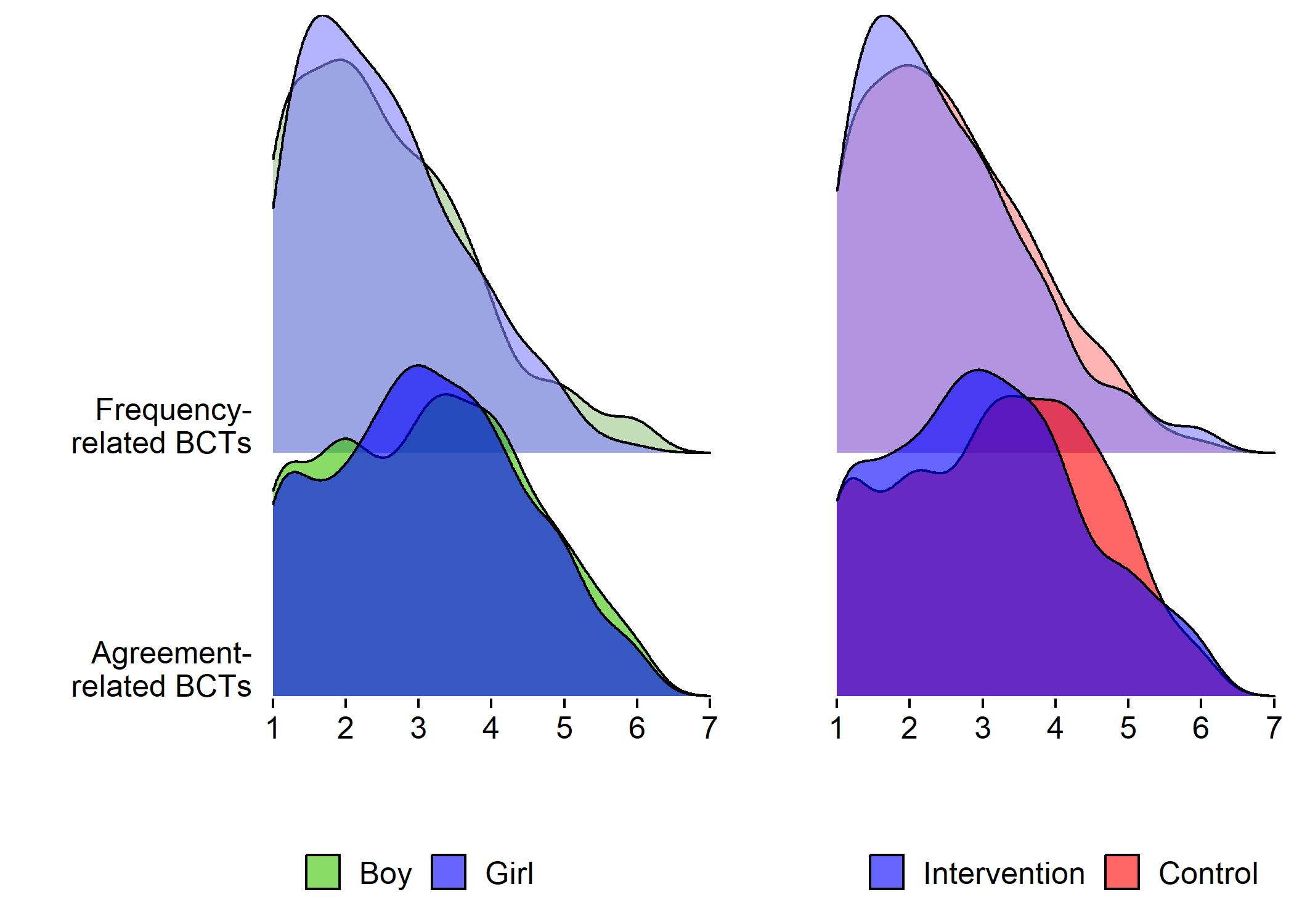
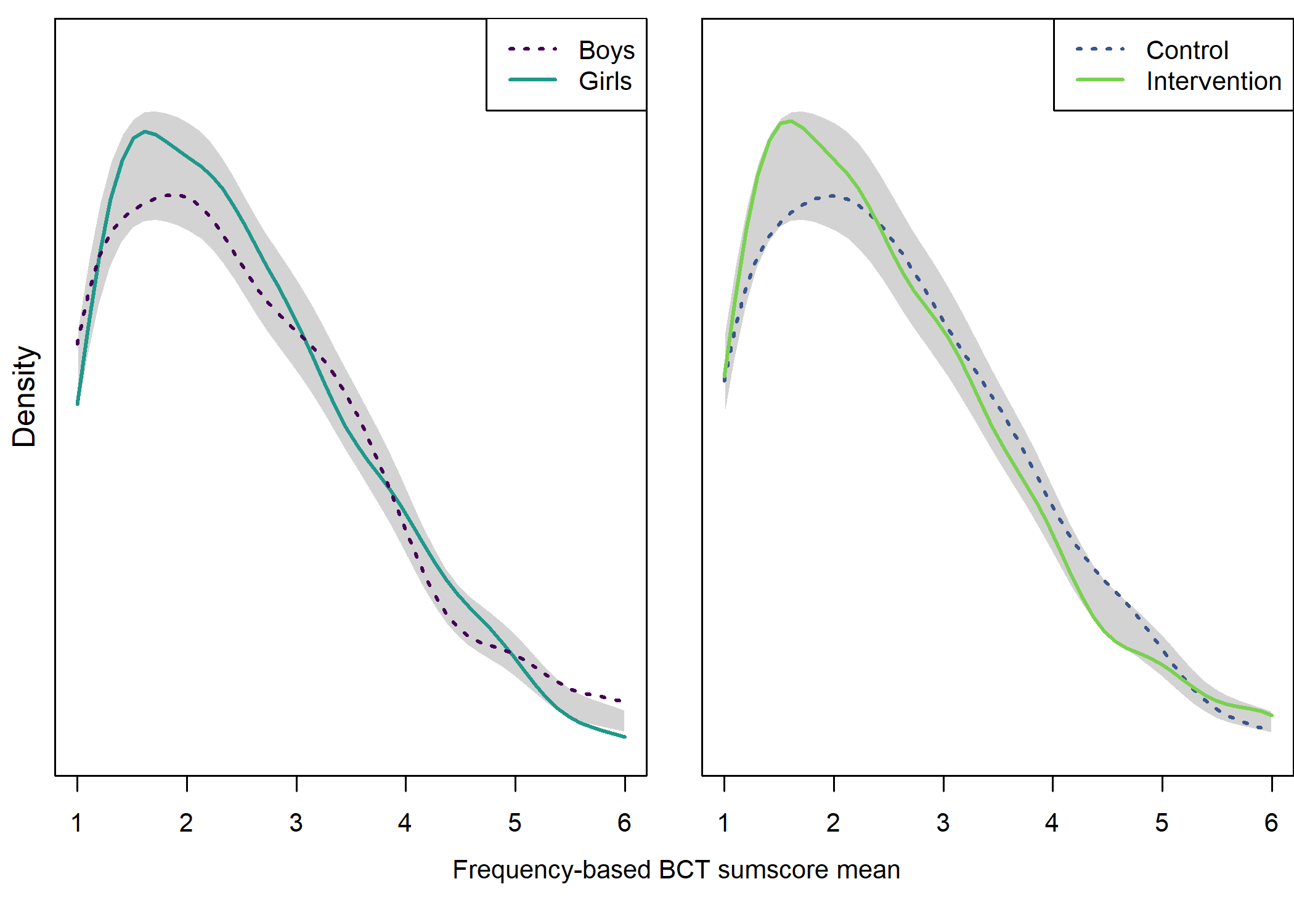
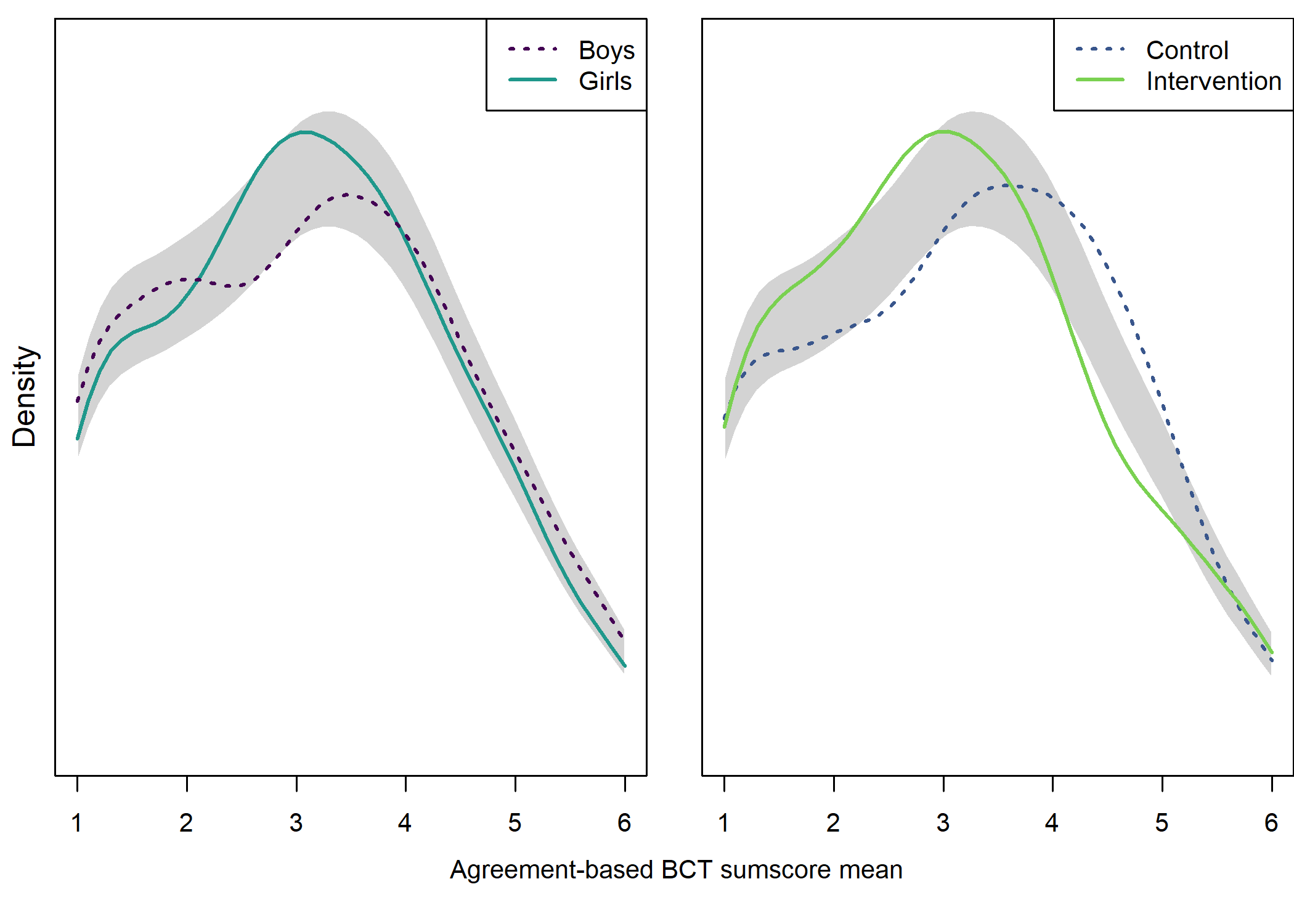
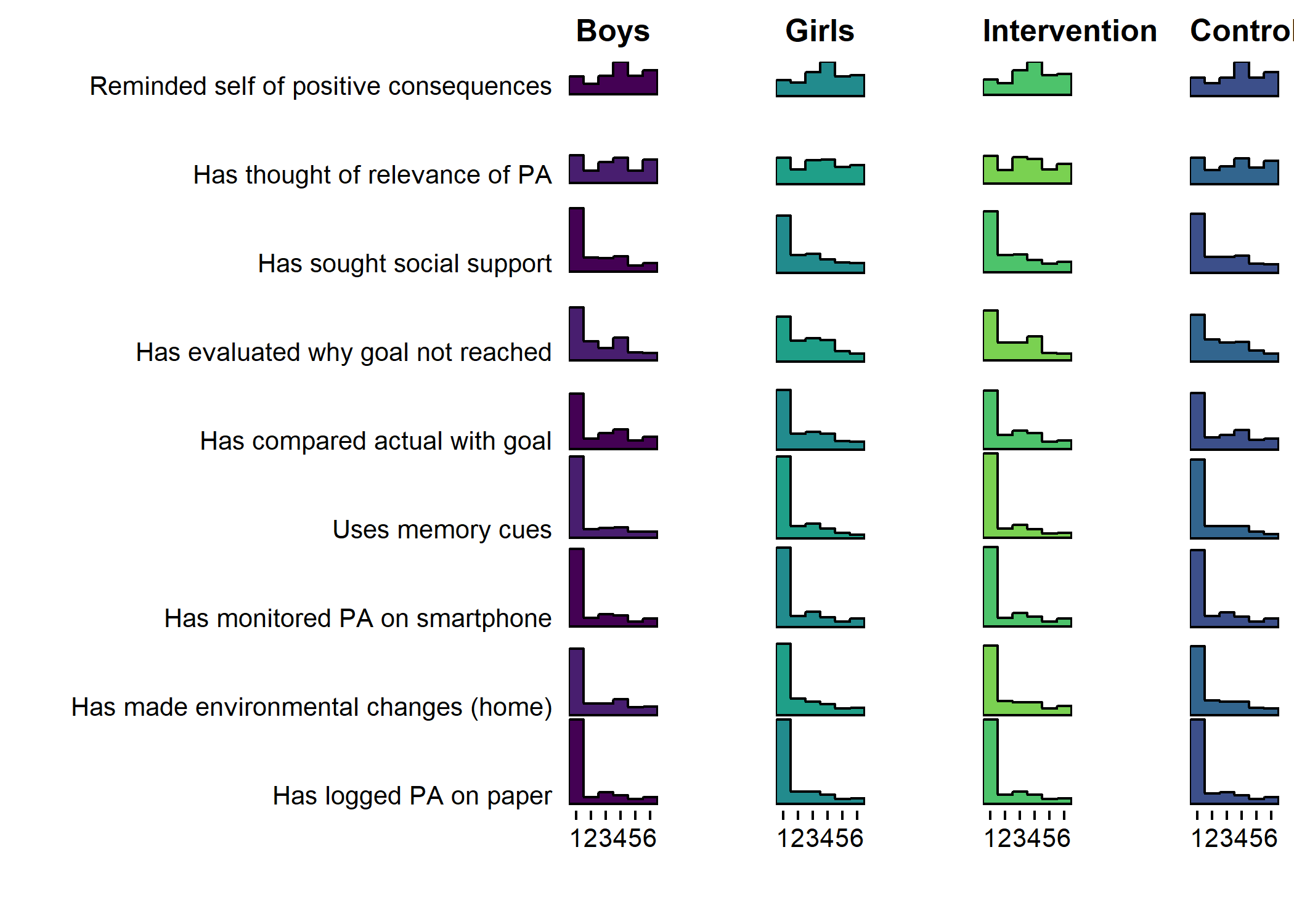
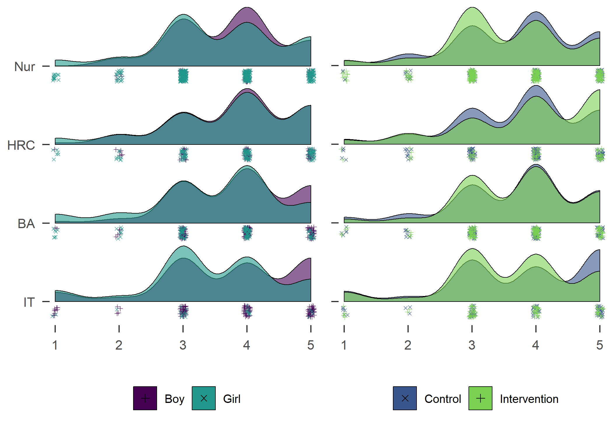
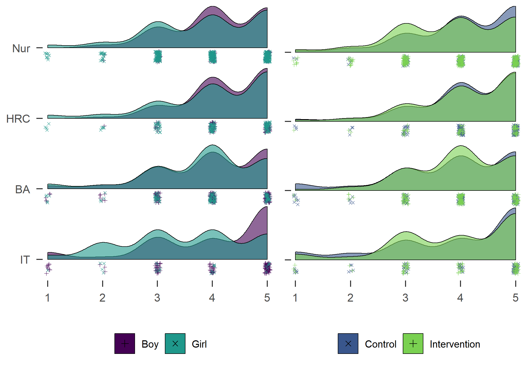
Introduction

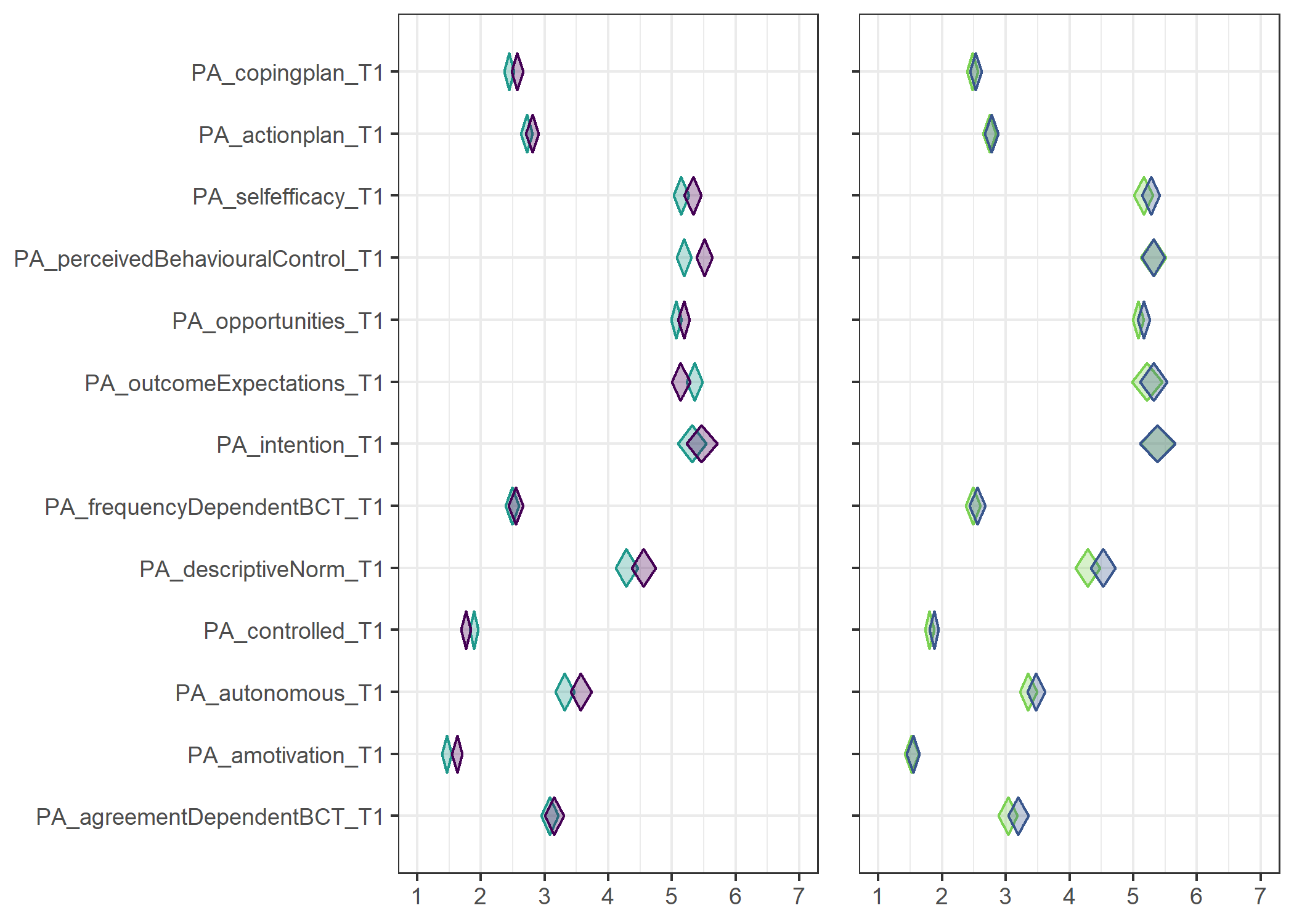
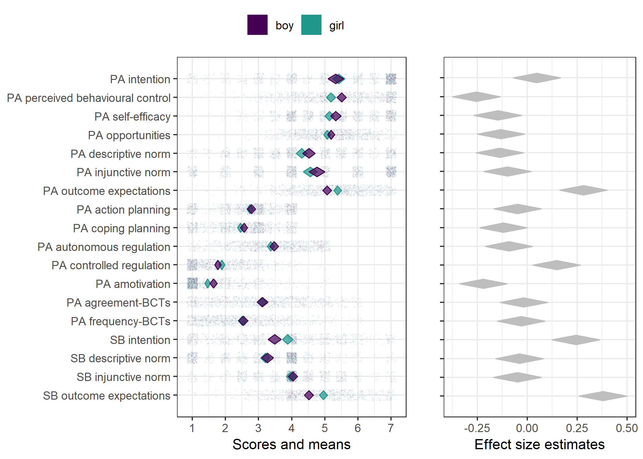
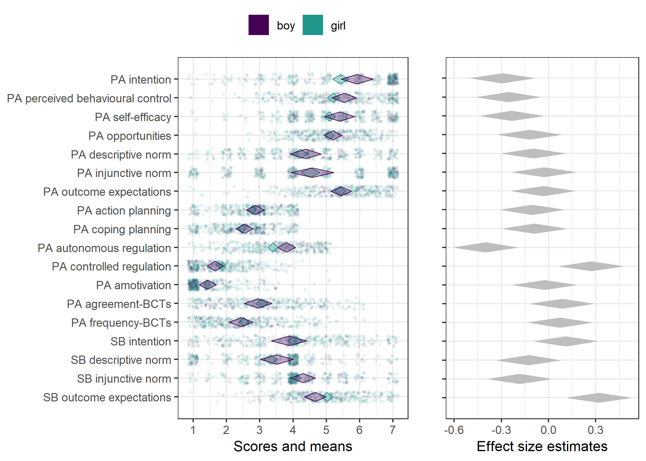
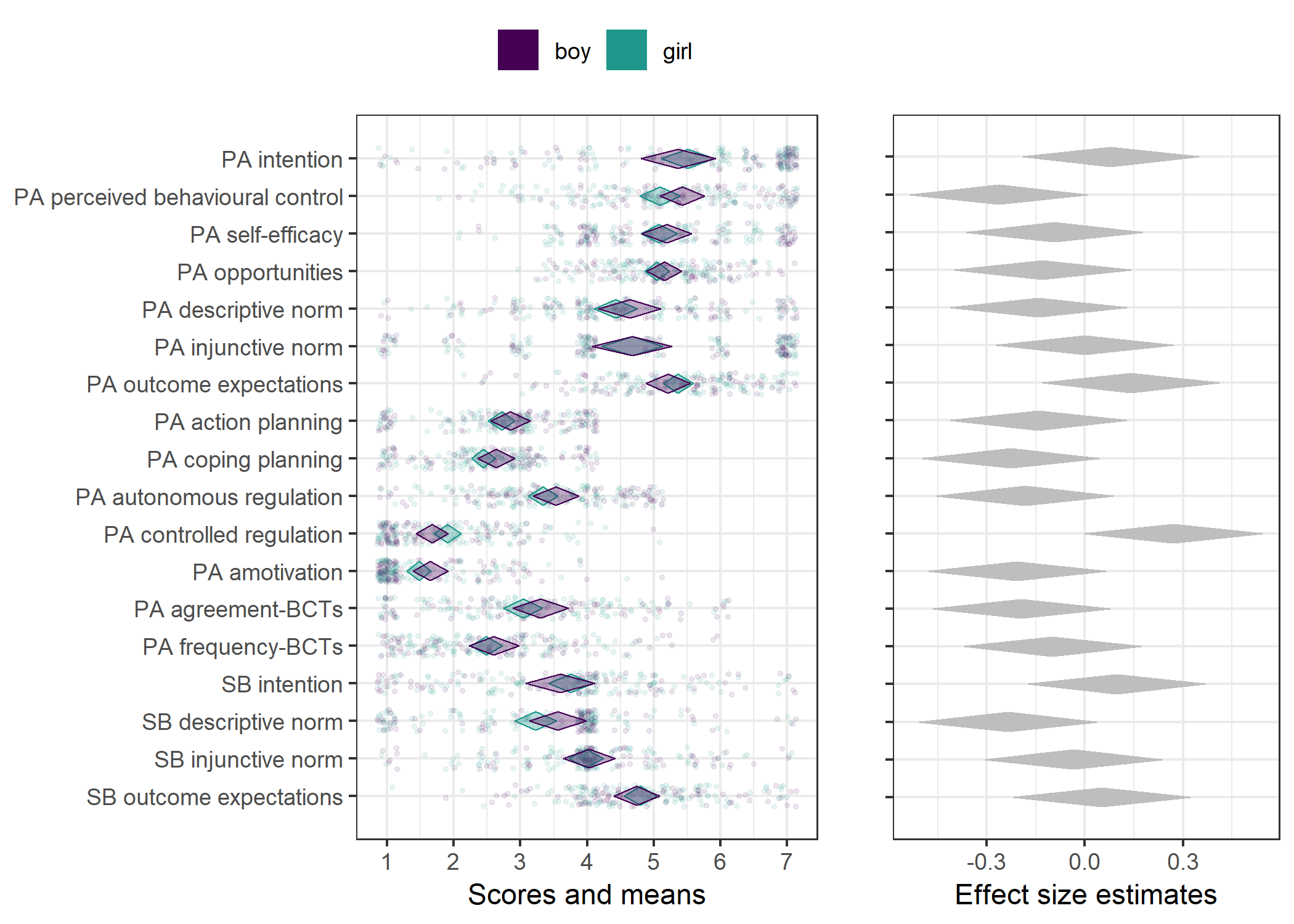
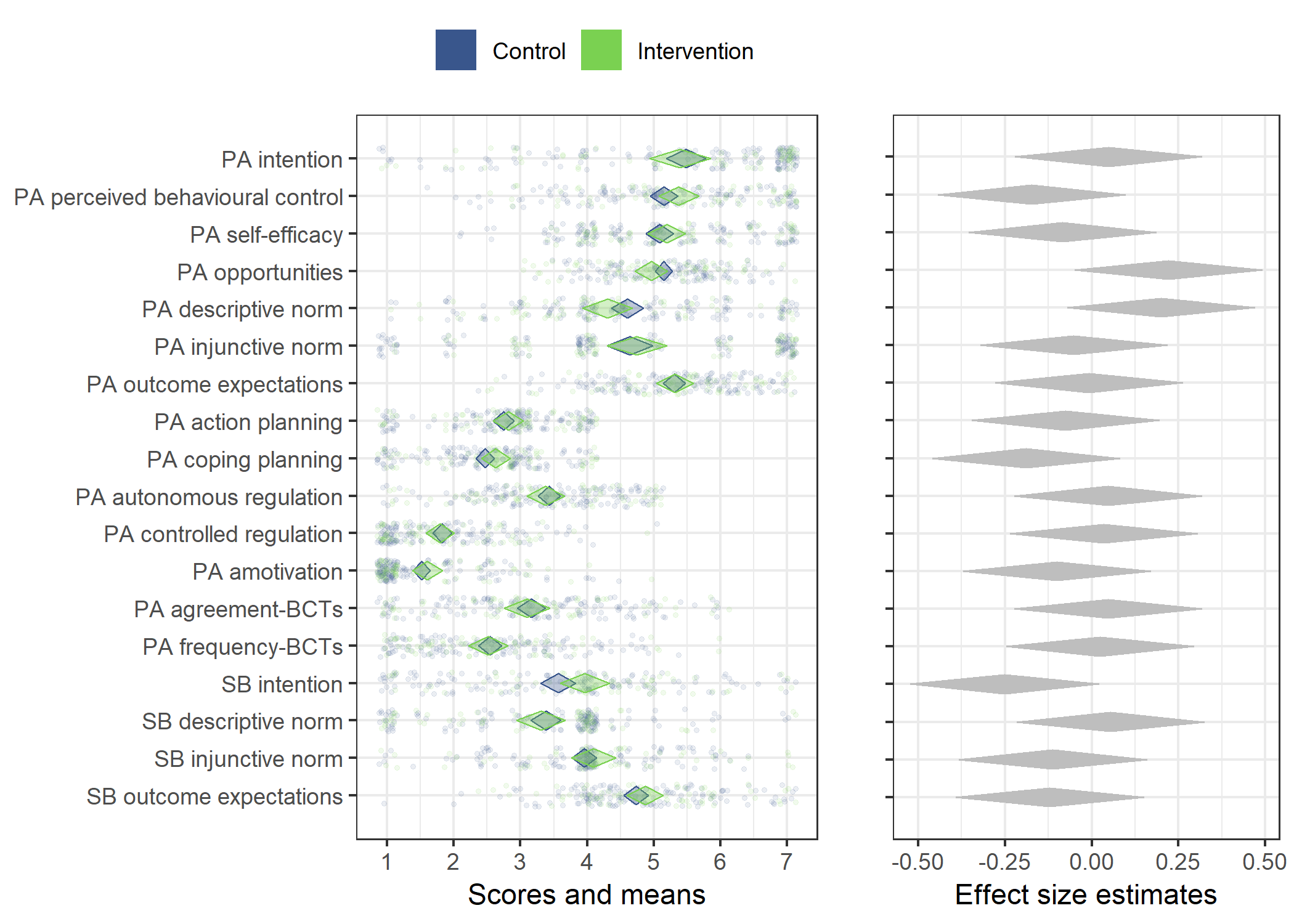
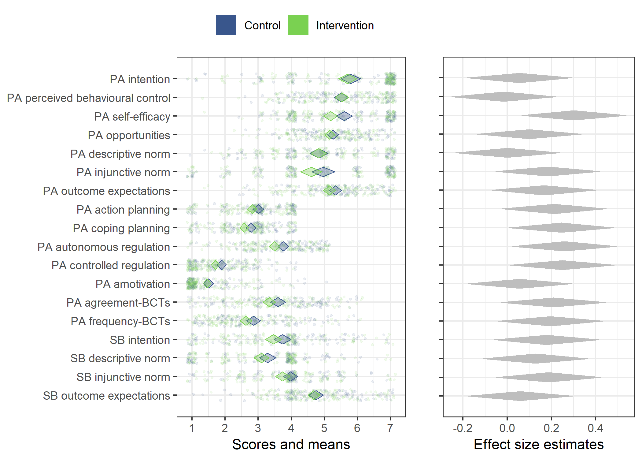
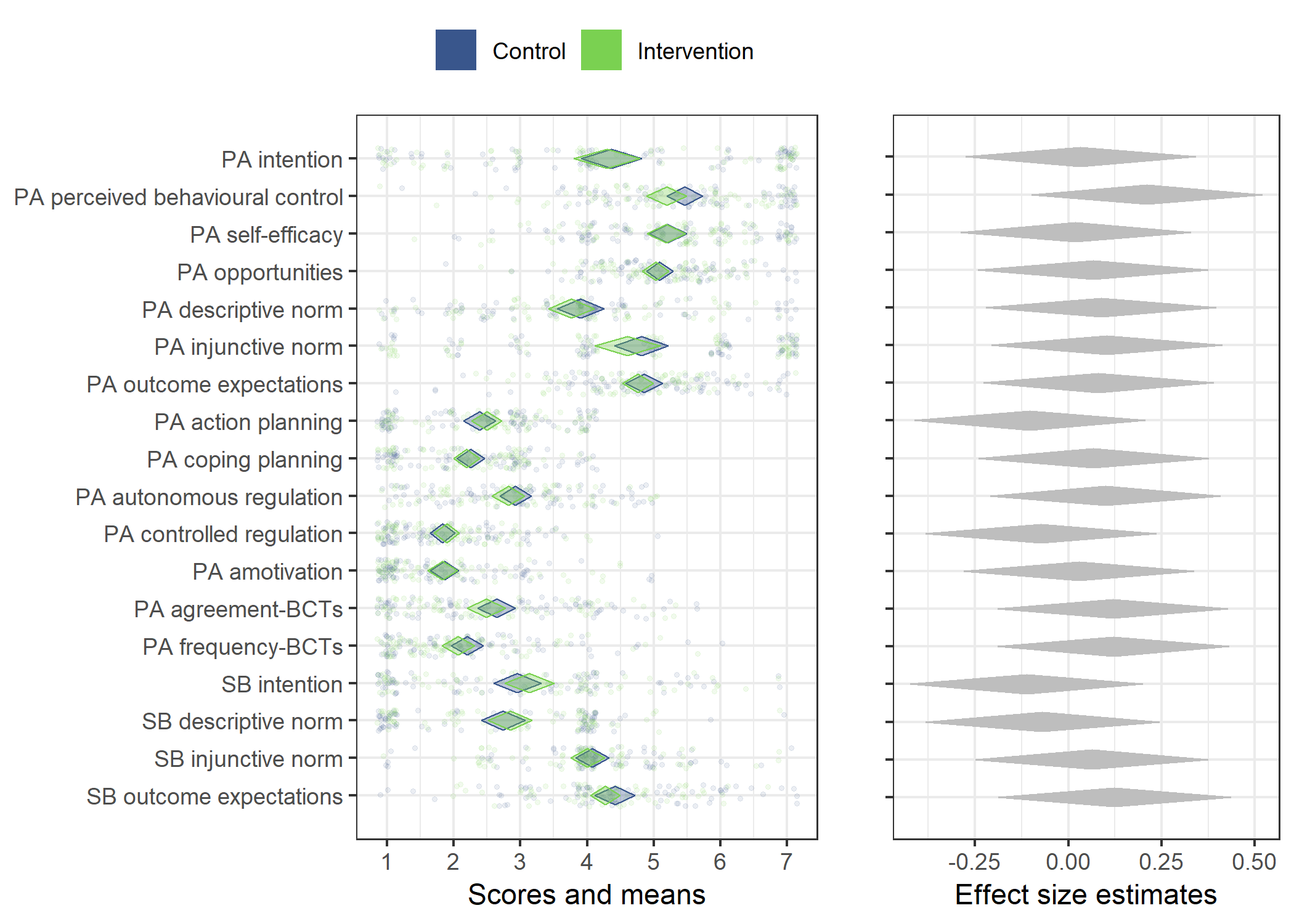
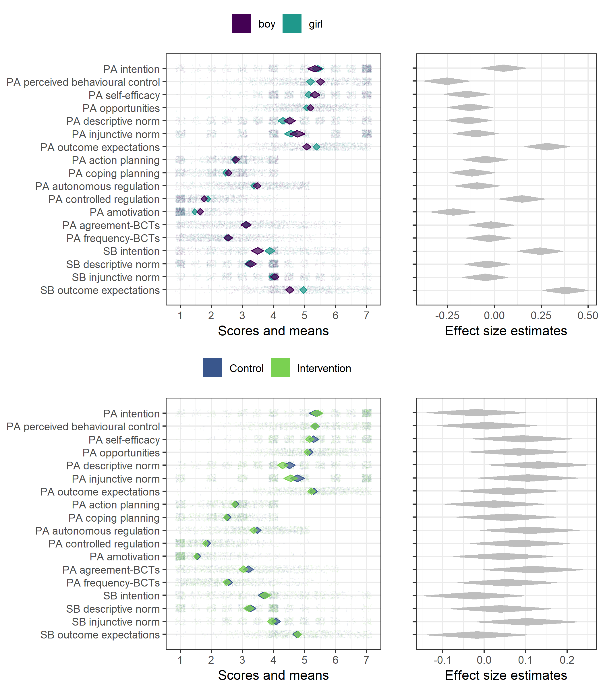
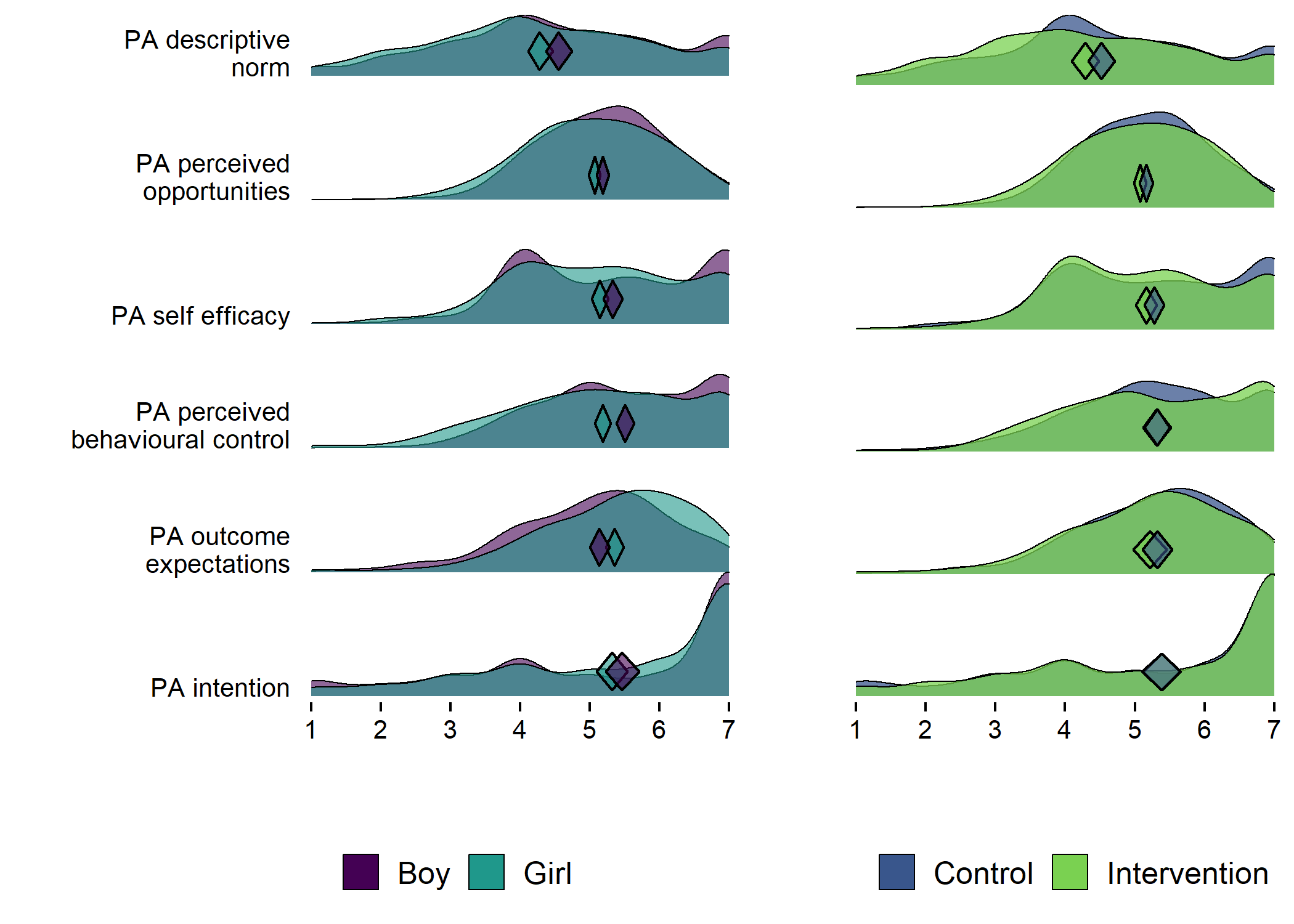
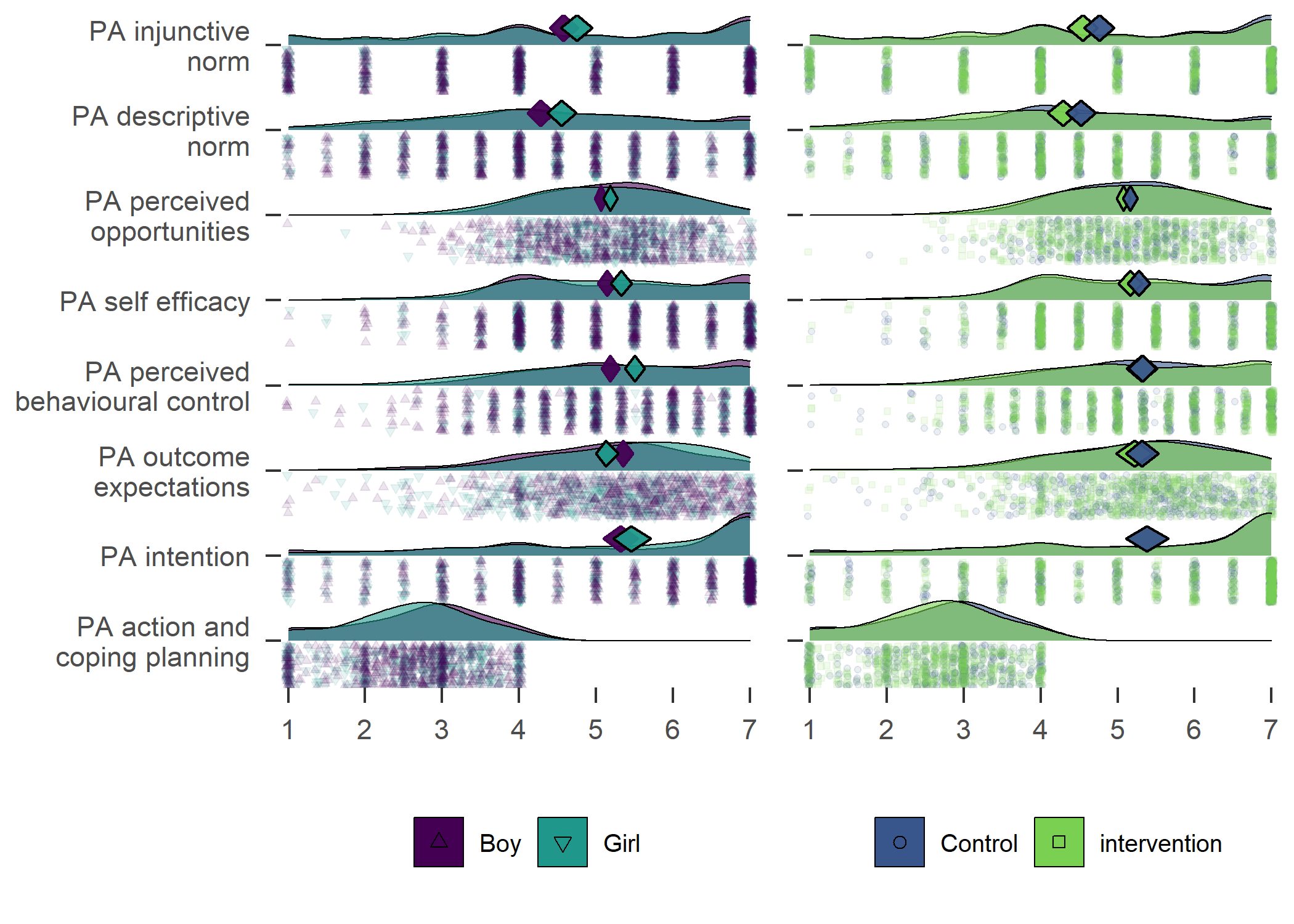
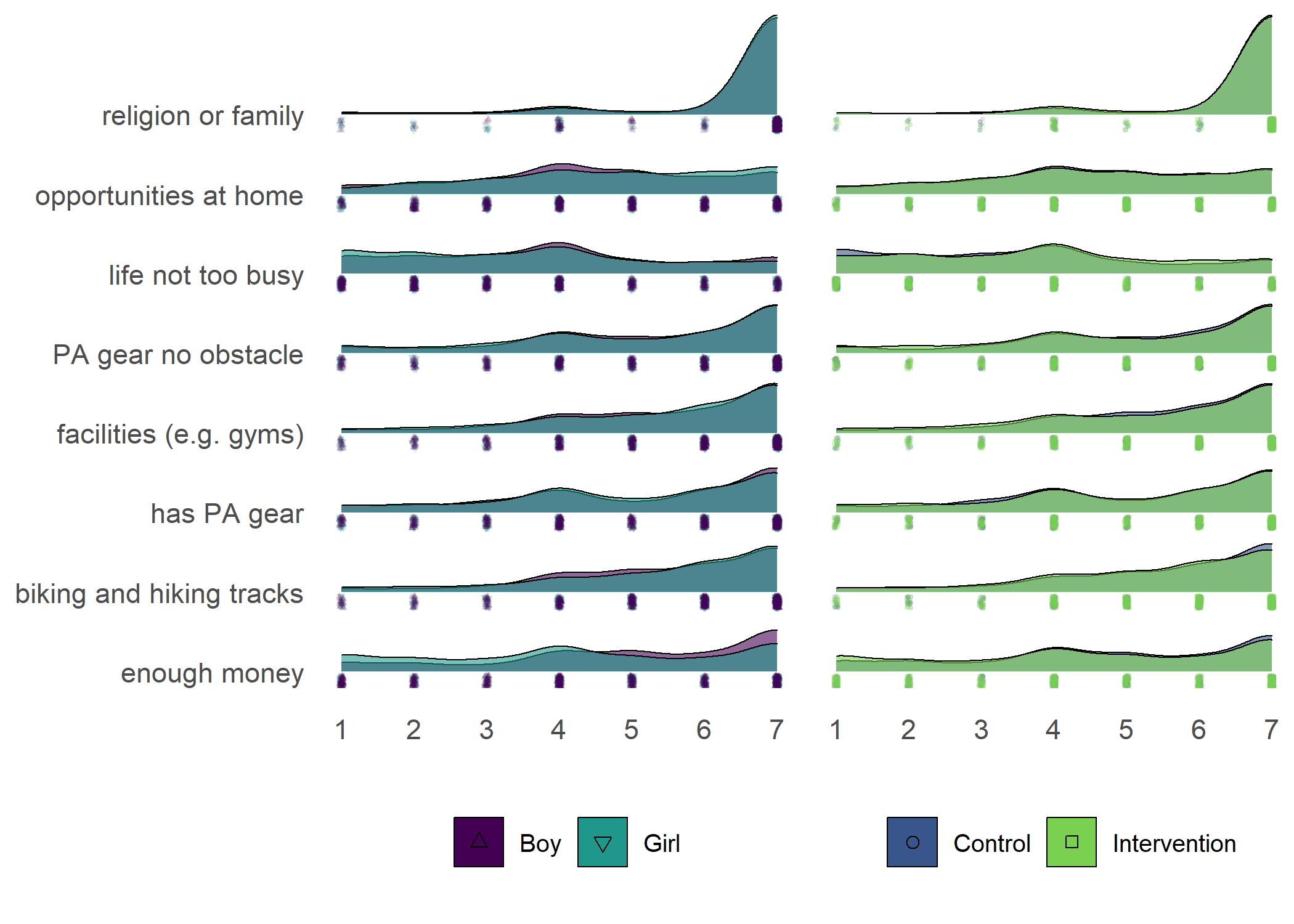
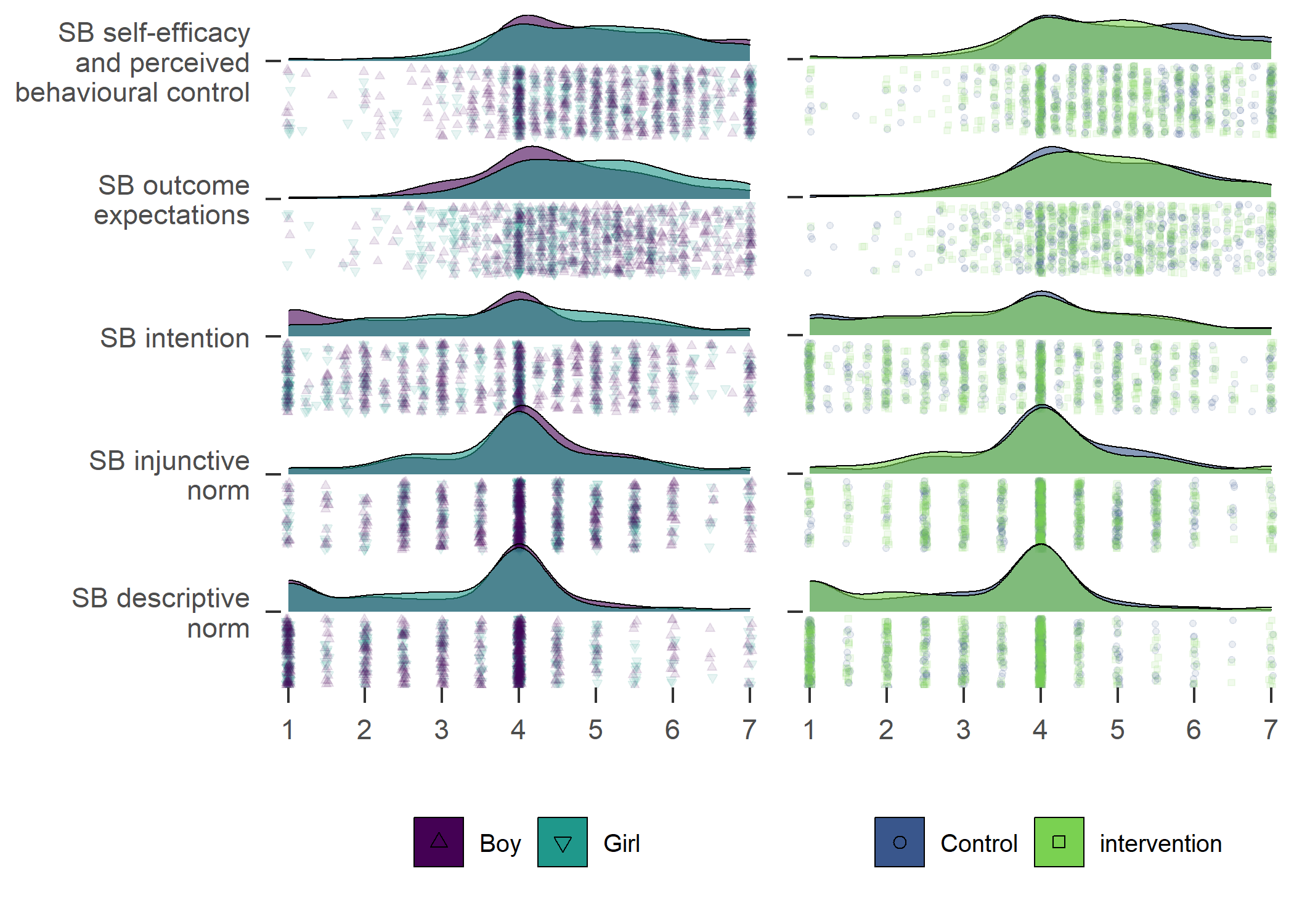
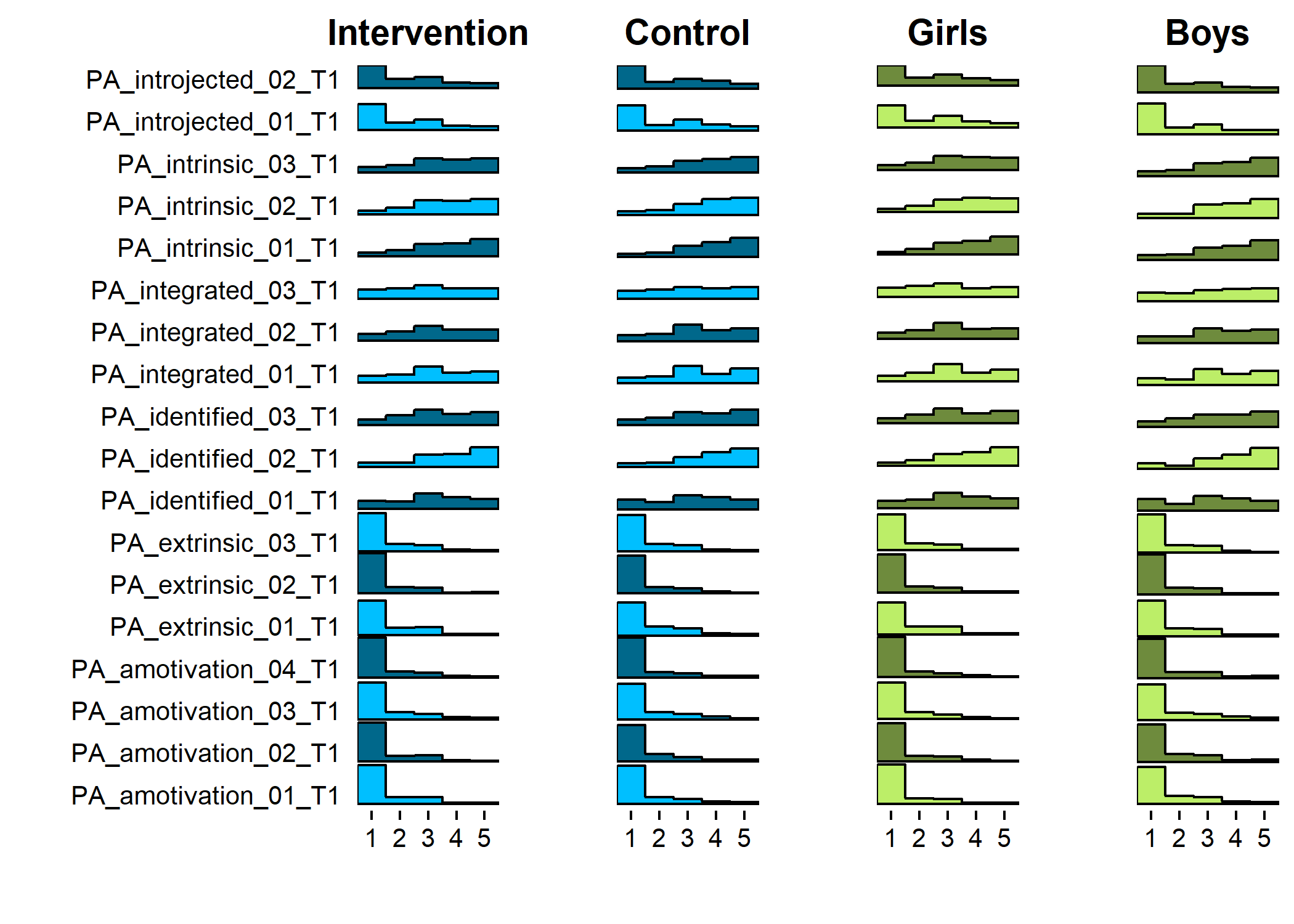
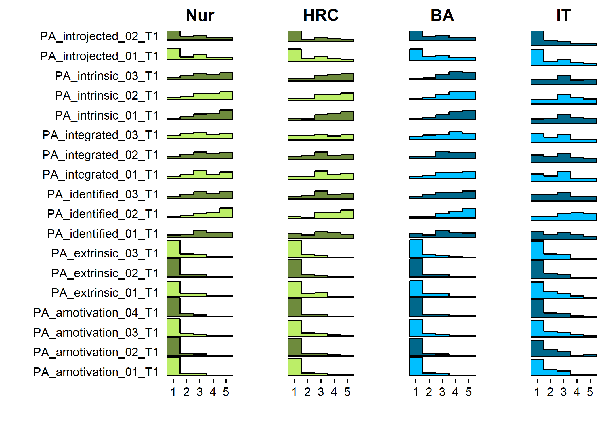
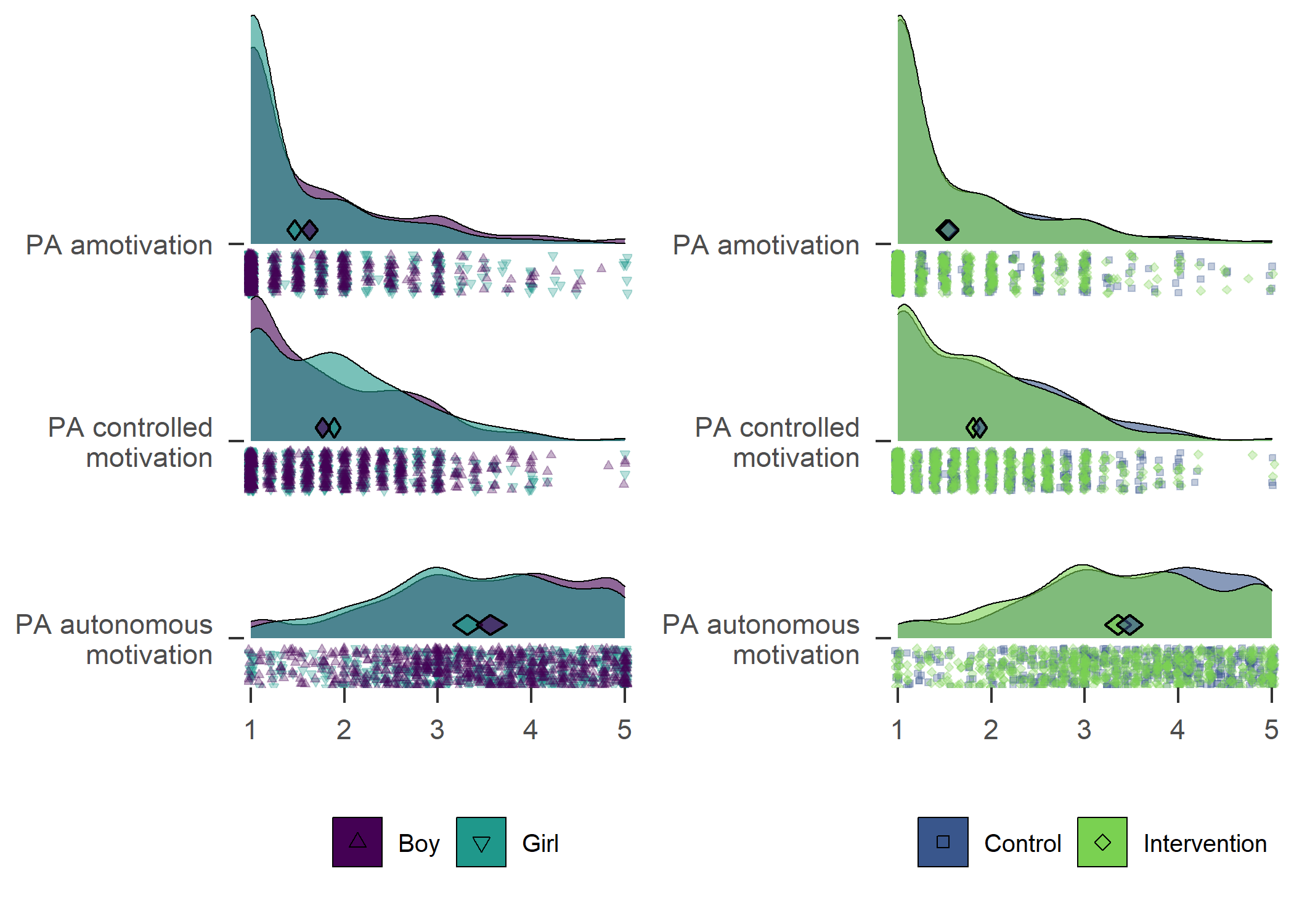
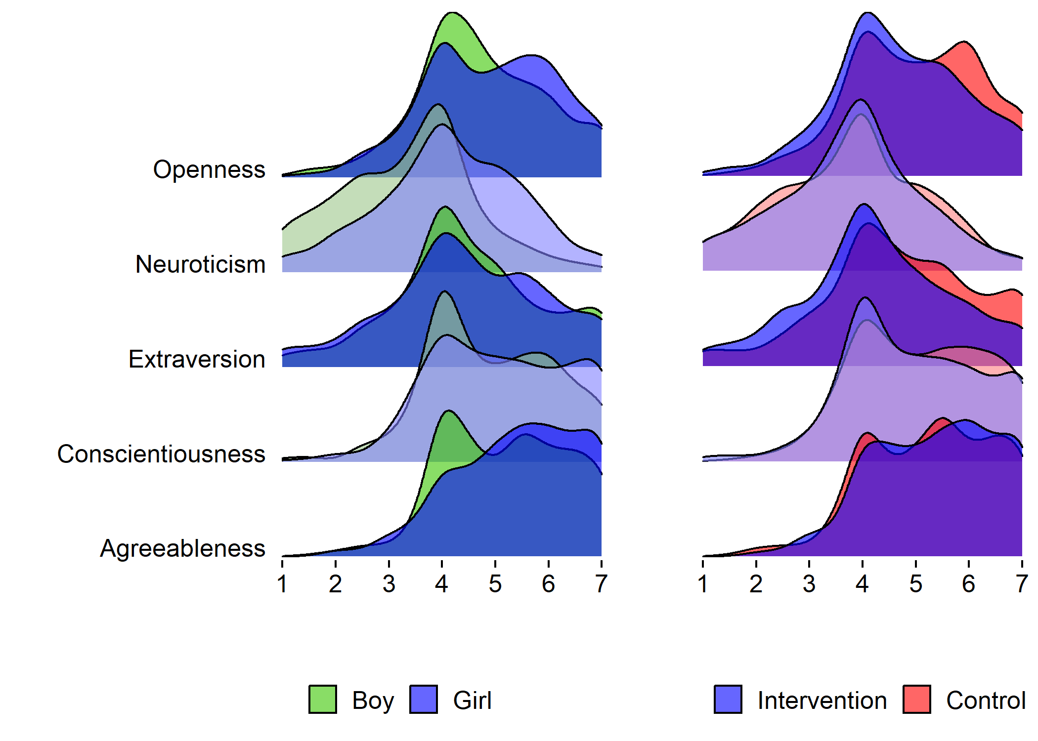
This section visualises distributions of variables, and describes the scales involved.

Clicking the “Code”-buttons on the right shows code for each chunk.

To start data analysis, we run a data compilation file to enable compiling the document. This file can be found here.

Note on using package brms

To use package brms (Bayesian Regression Models using ‘Stan’) you need RStan and Rtools, and to manually set Rtools folder if it’s not C:/Rtools/.

Description of accelerometer measurement

The hip-worn accelerometer (Hookie AM 20, Traxmeet Ltd, Espoo, Finland) using a digital triaxial acceleration sensor (ADXL45; Analog Devices, Norwood MA) was attached to a flexible belt and participants were instructed to wear the belt around their right hip for seven consecutive days during waking hours, except during shower and other water activities. The acceleration signal was collected at 100 Hz sampling frequency, ± 16 g acceleration range and 0.004 g resolution. PA-parameters were based on mean amplitude deviation (MAD) of the resultant acceleration analysed in 6s epochs [1]. The MAD values were then converted to metabolic equivalent (MET) values [2]. The epoch-wise MET values were further smoothed by calculating 1min exponential moving average. Using the smoothed MET values total PA was classified in terms of energy consumption covering MET values higher than 1.5 and moderate-to-vigorous PA (MVPA) covering MET values equal to or higher than 3 [1,2]. According to the definition of SB [3], time spent in sitting and reclining positions were combined to indicate SB, whereas standing was analysed separately as another form of stationary behaviour. Body postures were recognised from the raw acceleration data by employing both direction and intensity information from all three measurement axes. The recognition was based on the low intensity of movement (<1.5 MET) and the accelerometer orientation in relation to identified upright position (angle for posture estimation, APE) calculated at the end of each 6 s epoch [4].

  1. Vähä-Ypyä H, Vasankari T, Husu P, Suni J, Sievänen H. A universal, accurate intensity-based classification of different physical activities using raw data of accelerometer. Clinical physiology and functional imaging. 2015;35:64–70.
  2. Vähä-Ypyä H, Vasankari T, Husu P, Mänttäri A, Vuorimaa T, Suni J, et al. Validation of cut-points for evaluating the intensity of physical activity with accelerometry-based mean amplitude deviation (MAD). PLoS One. 2015;10:e014813.
  3. Tremblay MS, Aubert S, Barnes JD, Saunders TJ, Carson V, Latimer-Cheung AE, et al. Sedentary Behavior Research Network (SBRN) – Terminology Consensus Project process and outcome. International Journal of Behavioral Nutrition and Physical Activity. 2017;14:75. Available from: https://doi.org/10.1186/s12966-017-0525-8
  4. Vähä-Ypyä H, Husu P, Suni J, Vasankari T, Sievänen H. Reliable recognition of lying, sitting, and standing with a hip-worn accelerometer. Scand J Med Sci Sports. 2018;28:1092–102.

Descriptions of scales used to measure main theoretical predictors of PA

All scales, their properties and individual items can be found in the codebook.

Outcome expectations. Outcome expectations were measured using a 12-item scale, with the items based on a belief elicitation study conducted in the study population, in line with standard procedures (Francis et al., 2004). The scale consisted of 9 positive outcome expectations items and three negative ones.

Autonomous motivation. We used 15 items from the 19-item BREQ-2 questionnaire (Markland & Tobin, 2004), combined with three items from the integrated regulation scale from Wilson et al. (2006).

Perceived environmental opportunities. Environmental and social opportunities for PA were measured using an 8-item scale developed for this study.

Descriptive norms. PA descriptive norm was gauged by two questions, one on the behaviour of friends and the other on the behaviour of parents.

Intention. Participants were queried about their intention to be physically active with two questions. Both were formed as “I intend to be physically active for at least 1,5 hours weekly, during the next month”. Both had a scale from 1 to 7, the first ranging from “unlikely” to “likely” and the other ranging from “absolutely not” to “absolutely yes”.

Action- and coping planning. Action- and coping planning was measured with an 8-item scale (Sniehotta et al., 2005).

Self-efficacy/perceived behavioural control. PA self-efficacy was measured with 2 items, perceived behavioural control with 3 items (Hagger et al., 2003).

Behaviour change technique (BCT) use:

Use of BCTs was assessed by asking whether the participants had engaged in them during the last three weeks. The scale was not previously validated, but was used in (improved from?) the feasibility study (Hankonen et al 2017). Two types of BCTs were assessed; those judged to benefit from repeated enactment (such as reminding oneself of positive consequences) and others, such as goal setting.

Agreement-dependent BCTs.

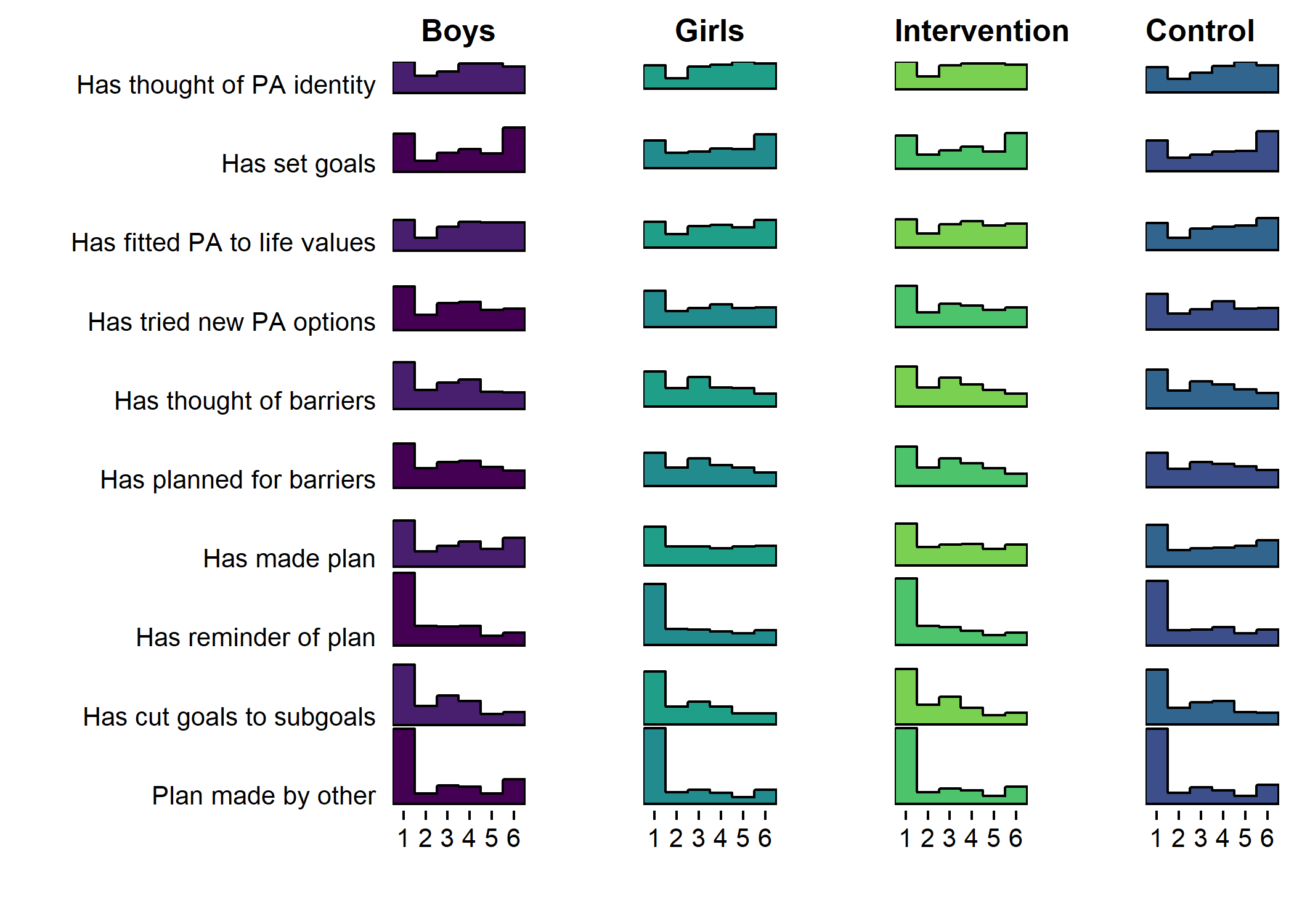
Agreement-dependent BCTs were asked with the lead “Have you done the following during the last three weeks?”. The response scale ranged from 1 = not at all true to 6 = completely true. Items are as follows:

  1. I have set PA goals for myself.
  2. I have personally made a specific plan (“what, where, how”) to implement my PA.
  3. I have a PA plan, which has been made by someone else, e.g. my sports club (e.g. a workout schedule).
  4. I have a way by which I remind myself of my PA plan, e.g. I write it down in the calendar.
  5. I have broken down larger PA goals to smaller subgoals.
  6. I have tried out new ways for me to be physically active.
  7. I have pondered, what kind of difficult situations or barriers prevent me from implementing my PA plan.
  8. I have planned for ways to overcome barriers to doing PA.
  9. I have thought about how PA fits my identity (self concept).
  10. I have attempted to find ways to exercise so, that it won’t obstruct but instead helps actualise my other life values.

Frequency-dependent BCTs.

The answer scale for frequency-dependent BCTs was as follows: 1 = not once, 2 = once, 3 = twice, 4 = weekly, 5 = about every second day, 6 = daily. Items are as follows:

  1. I have reminded myself in my spare time what kind of positive consequences frequent PA would have in my life.
  2. I have monitored my PA by marking the PA occasions on an exercise log on paper.
  3. I have monitored my PA by using a smartphone, e.g. the Moves-app.
  4. I have used memory cues with which I remember to implement my PA intention.
  5. I have compared my actualized PA with the PA goal I have set.
  6. I have thought about which reasons to do PA are important to me personally.
  7. I have made changes in my home (e.g. my room or my computer), so that starting PA would be easier.
  8. I have asked my friends or family for support to reach my PA goals.
  9. If I haven’t reached my PA goal, I have evaluated, what went wrong.

\(~\) \(~\)

Average day’s activity as proportions

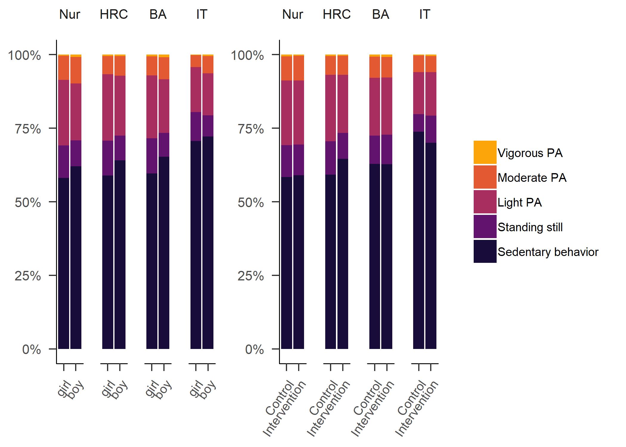
These plots show the average proportions of daily activity by gender and intervention. Note, that they hide the variability in these values.

Stacking raw values


averageDayActivityPlot_gender <- df %>%  
  dplyr::select(girl, intervention, track,
                     "Sedentary behavior" = sitLieAccelerometer_T1, 
                     "Standing still" = standingAccelerometer_T1, 
                     "Light PA" = lpaAccelerometer_T1, 
                     "Moderate PA" = mpaAccelerometer_T1, 
                     "Vigorous PA" = vpaAccelerometer_T1) %>%
  dplyr::filter(track != "Other") %>% # Drop small track "Other"
  tidyr::gather(variable, value, -(girl:track)) %>% # Convert data to long form
  dplyr::mutate(track = factor(track, ordered = TRUE,
                               levels = c("Nur",
                                          "HRC",
                                          "BA",
                                          "IT",
                                          "Other")), # Order factors, to preserve presentation order
                variable = factor(variable, ordered = TRUE,
                                  levels = c("Sedentary behavior", 
                                             "Standing still", 
                                             "Light PA", 
                                             "Moderate PA", 
                                             "Vigorous PA"))) %>% 
  ggplot2::ggplot(aes(y = value, x = girl)) +
  # coord_flip() +
  geom_bar(aes(fill = variable), 
           position = position_fill(reverse = TRUE),
           stat = "identity") +
  scale_y_continuous(labels = scales::percent) +
  scale_fill_viridis_d(option = "inferno", begin = 0.1, end = 0.8) +
  labs(x = NULL, y = NULL) +
  theme(legend.title=element_blank()) +
  guides(fill = guide_legend(reverse = TRUE)) + # Make the legend order match the plot order
  facet_wrap("track", nrow = 1)

# Same plot but for intervention/control:

averageDayActivityPlot_intervention <- df %>% dplyr::select(girl, intervention, track,
                     "Sedentary behavior" = sitLieAccelerometer_T1, 
                     "Standing still" = standingAccelerometer_T1, 
                     "Light PA" = lpaAccelerometer_T1, 
                     "Moderate PA" = mpaAccelerometer_T1, 
                     "Vigorous PA" = vpaAccelerometer_T1) %>%
  dplyr::filter(track != "Other") %>% # Drop small track "Other"
  tidyr::gather(variable, value, -(girl:track)) %>% # Convert data to long form
  dplyr::mutate(track = factor(track, ordered = TRUE,
                               levels = c("Nur",
                                          "HRC",
                                          "BA",
                                          "IT",
                                          "Other")), 
                variable = factor(variable, ordered = TRUE,
                                  levels = c("Sedentary behavior", 
                                             "Standing still", 
                                             "Light PA", 
                                             "Moderate PA", 
                                             "Vigorous PA")),
                intervention = factor(intervention, ordered = TRUE,
                                      levels = c(0, 1),
                                      labels = c("Control", "Intervention"))) %>% 
  ggplot2::ggplot(aes(y = value, x = intervention)) +
  # coord_flip() +
  geom_bar(aes(fill = variable), 
           position = position_fill(reverse = TRUE),
           stat = "identity") +
  scale_y_continuous(labels = scales::percent) +
  scale_fill_viridis_d(option = "inferno", begin = 0.1, end = 0.8) +
  labs(x = NULL, y = NULL) +
  theme(legend.title=element_blank(),
        axis.text.x = element_text(angle = 45, hjust = 1, size = 10)) + # Adjust label text
  guides(fill = guide_legend(reverse = TRUE)) + # Make the legend order match the plot order
  facet_wrap("track", nrow = 1)


averageDayActivityPlot_gender

Stacking percentages

In these plots, the time values are first converted to proportions for each participant. The function dplyr::mutate_at is used to take each variable which contains the word Accelerometer, but not those that contain the word weartime, and for each of those variables, a division by weartime is conducted.

As can be seen, the result is exactly the same, as when raw values were stacked.


averageDayActivityPlot_gender <- df %>% 
  dplyr::mutate_at(vars(contains("Accelerometer"), -contains("weartime")), funs(./weartimeAccelerometer_T1)) %>% 
  dplyr::select(girl, intervention, track,
                     "Sedentary behavior" = sitLieAccelerometer_T1, 
                     "Standing still" = standingAccelerometer_T1, 
                     "Light PA" = lpaAccelerometer_T1, 
                     "Moderate PA" = mpaAccelerometer_T1, 
                     "Vigorous PA" = vpaAccelerometer_T1) %>%
  dplyr::filter(track != "Other") %>% # Drop small track "Other"
  tidyr::gather(variable, value, -(girl:track)) %>% # Convert data to long form
  dplyr::mutate(track = factor(track, ordered = TRUE,
                               levels = c("Nur",
                                          "HRC",
                                          "BA",
                                          "IT",
                                          "Other")), # Order factors, to preserve presentation order
                variable = factor(variable, ordered = TRUE,
                                  levels = c("Sedentary behavior", 
                                             "Standing still", 
                                             "Light PA", 
                                             "Moderate PA", 
                                             "Vigorous PA"))) %>% 
  ggplot2::ggplot(aes(y = value, x = girl)) +
  # coord_flip() +
  geom_bar(aes(fill = variable), 
           position = position_fill(reverse = TRUE),
           stat = "identity") +
  scale_y_continuous(labels = scales::percent) +
  scale_fill_viridis_d(option = "inferno", begin = 0.1, end = 0.8) +
  labs(x = NULL, y = NULL) +
  theme(legend.position="none", 
        axis.text.x = element_text(angle = 55, hjust = 1, size = 10)) + # Adjust label text
  guides(fill = guide_legend(reverse = TRUE)) + # Make the legend order match the plot order
  facet_wrap("track", nrow = 1)

# Same plot but for intervention/control:

averageDayActivityPlot_intervention <- df %>% 
  dplyr::mutate_at(vars(contains("Accelerometer"), -contains("weartime")), funs(./weartimeAccelerometer_T1)) %>% 
  dplyr::select(girl, intervention, track,
                     "Sedentary behavior" = sitLieAccelerometer_T1, 
                     "Standing still" = standingAccelerometer_T1, 
                     "Light PA" = lpaAccelerometer_T1, 
                     "Moderate PA" = mpaAccelerometer_T1, 
                     "Vigorous PA" = vpaAccelerometer_T1) %>% 
  dplyr::filter(track != "Other") %>% # Drop small track "Other"
  tidyr::gather(variable, value, -(girl:track)) %>% # Convert data to long form
  dplyr::mutate(track = factor(track, ordered = TRUE,
                               levels = c("Nur",
                                          "HRC",
                                          "BA",
                                          "IT",
                                          "Other")), 
                variable = factor(variable, ordered = TRUE,
                                  levels = c("Sedentary behavior", 
                                             "Standing still", 
                                             "Light PA", 
                                             "Moderate PA", 
                                             "Vigorous PA")),
                intervention = factor(intervention, ordered = TRUE,
                                      levels = c(0, 1),
                                      labels = c("Control", "Intervention"))) %>% 
  ggplot2::ggplot(aes(y = value, x = intervention)) +
  # coord_flip() +
  geom_bar(aes(fill = variable), 
           position = position_fill(reverse = TRUE),
           stat = "identity") +
  scale_y_continuous(labels = scales::percent) +
  scale_fill_viridis_d(option = "inferno", begin = 0.1, end = 0.8) +
  labs(x = NULL, y = NULL) +
  theme(legend.title=element_blank(),
        axis.text.x = element_text(angle = 55, hjust = 1, size = 10)) + # Adjust label text
  guides(fill = guide_legend(reverse = TRUE)) + # Make the legend order match the plot order
  facet_wrap("track", nrow = 1)


averageDayActivityPlot_gender +
averageDayActivityPlot_intervention

Primary outcome variables

[code chunk below transforms MVPA, SB and wear time to hours for ease of interpretation]

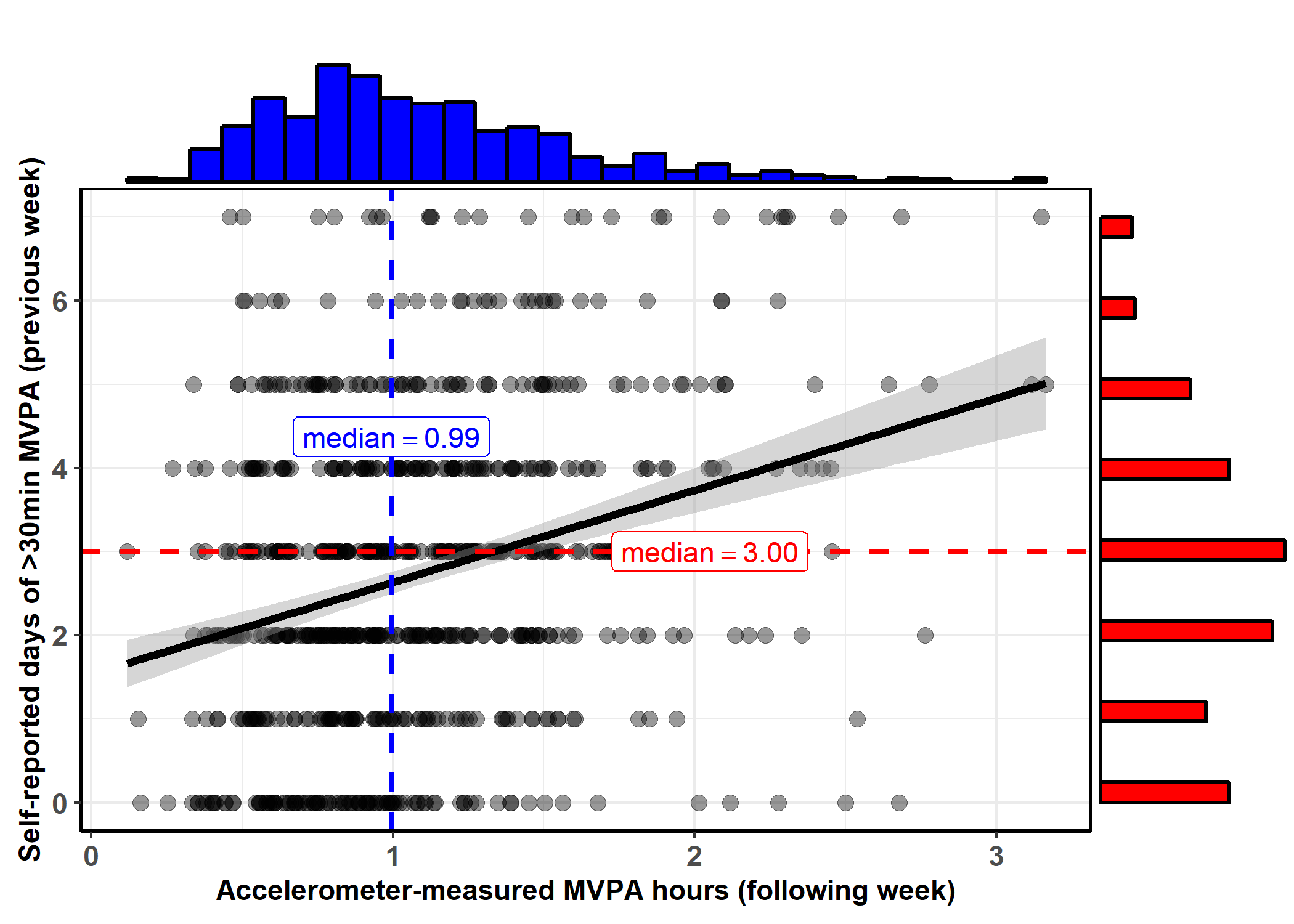
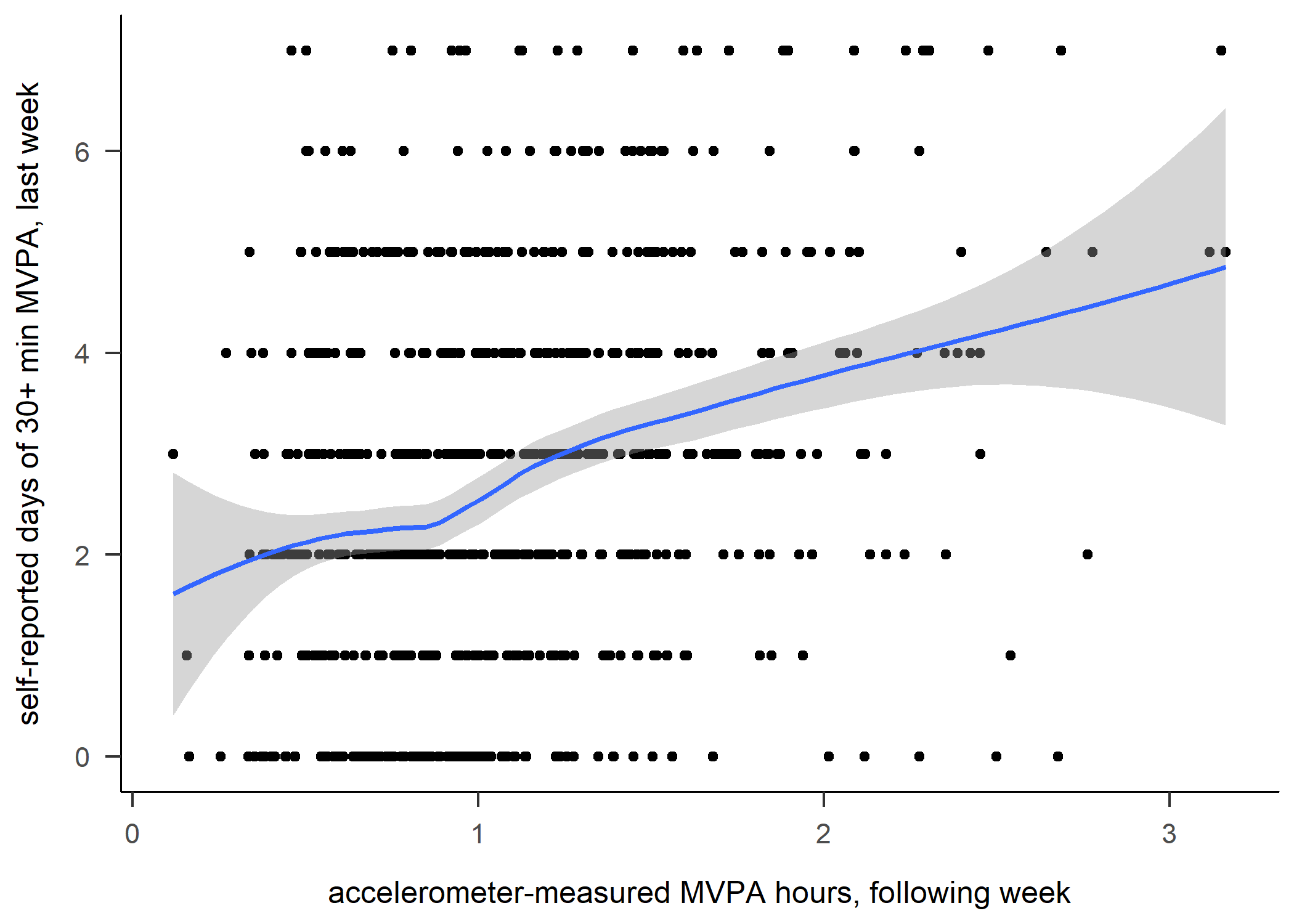
Self-reported vs. accelerometer-measured MVPA

Accelerometer weartime

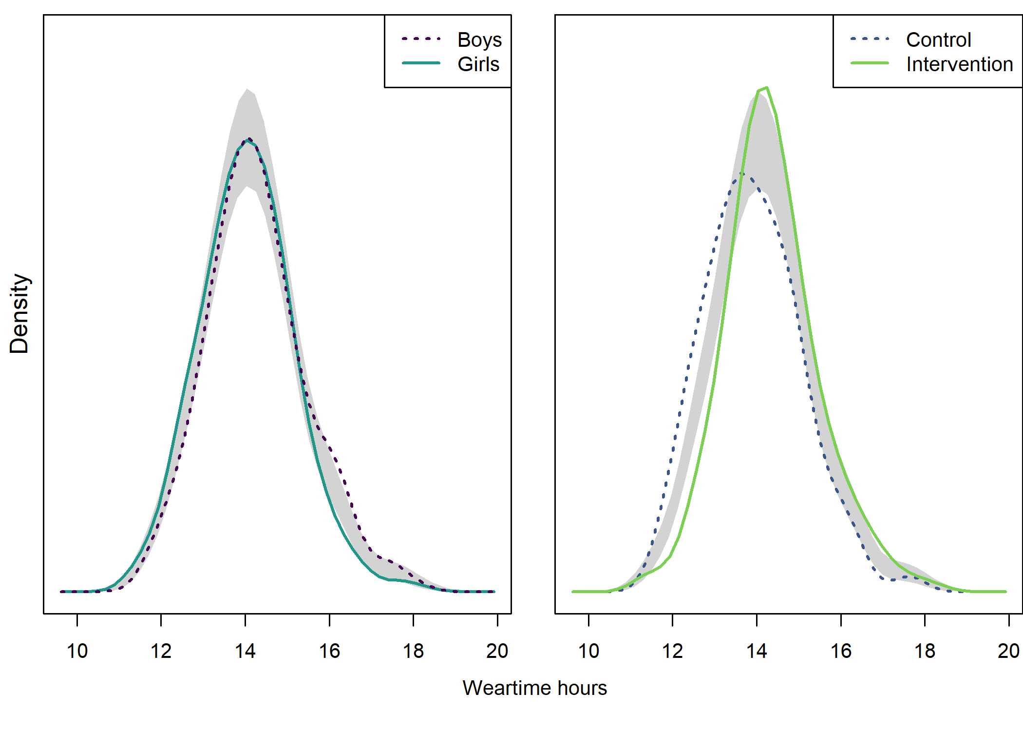
Density plot by intervention and gender


# Create data frame
densplot <- d
levels(densplot$intervention) <- c("Control", "Intervention")
levels(densplot$girl) <- recode(densplot$girl, "boy" = "Boys", "girl" = "Girls")

# This gives side-by-side plots. There's a third plot below the two, which is fake to include x-axis text.
layout(matrix(c(1, 2, 3, 3), nrow = 2, ncol = 2, byrow = TRUE),
       widths = c(0.5, 0.5), heights = c(0.45, 0.05))

# Minimise whitespace; see https://stackoverflow.com/questions/15848942/how-to-reduce-space-gap-between-multiple-graphs-in-r
par(mai = c(0.3, 0.3, 0.1, 0.0)) 

## Girls vs. boys
# Choose only the variables needed and drop NA
dens <- densplot %>% dplyr::select(weartimeAccelerometer_T1, girl) %>% 
  dplyr::filter(complete.cases(.))

# Set random number generator for reproducibility of bootstrap test of equal densities
set.seed(10)

# Make plot
sm.weartimeAccelerometer_T1_2 <- sm.density.compare2(as.numeric(dens$weartimeAccelerometer_T1), 
                                               as.factor(dens$girl), 
                                               model = "equal",
                                               xlab = "", ylab = "",
                                               col = viridis::viridis(4, end  =  0.8)[c(3, 1)], 
                                               lty = c(1,3), yaxt = "n",
                                               bandcol = 'LightGray', 
                                               lwd = (c(2,2)))
## 
## Test of equal densities:  p-value =  0.41
legend("topright", levels(dens$girl), col = viridis::viridis(4, end = 0.8)[c(1, 3)], lty = c(3,1), lwd = (c(2,2)))
mtext(side = 2, "Density", line = 0.5)

## Intervention vs. control
# Choose only the variables needed and drop NA
dens <- densplot %>% dplyr::select(weartimeAccelerometer_T1, intervention) %>% 
  dplyr::filter(complete.cases(.))

# Set random number generator for reproducibility of bootstrap test of equal densities
set.seed(10)
# Make plot
sm.weartimeAccelerometer_T1_2 <- sm.density.compare2(as.numeric(dens$weartimeAccelerometer_T1), 
                                               as.factor(dens$intervention), 
                                               model = "equal", 
                                               xlab = "", ylab = "",
                                               col = viridis::viridis(4, end = 0.8)[c(2, 4)], 
                                               lty = c(3,1), yaxt = "n",
                                               bandcol = 'LightGray', 
                                               lwd = (c(2,2)))
## 
## Test of equal densities:  p-value =  0
legend("topright", levels(dens$intervention), col = viridis::viridis(4, end = 0.8)[c(2, 4)], lty=c(3,1), lwd=(c(2,2)))

# Create x-axis label. See https://stackoverflow.com/questions/11198767/how-to-annotate-across-or-between-plots-in-multi-plot-panels-in-r
par(mar = c(0,0,0,0)) 
plot(1, 1, type = "n", frame.plot = FALSE, axes = FALSE) # Fake plot for x-axis label
text(x = 1.02, y = 1.3, labels = "Weartime hours", pos = 1)
Data preparation

Description

The tab “Information on data preparation” of this section present information on data preparation for the plot

Information on data preparation

Prepare data

# m_weartimeAccelerometer_trackgirl <- brms::bf(weartimeAccelerometer_T1 ~ (1 | track:girl)) %>% 
#   brms::brm(., data = df, chains = 4, iter = 4000, control = list(adapt_delta = 0.95))
# 
# brms::prior_summary(m_weartimeAccelerometer_trackgirl, data = df)
# 
# m_weartimeAccelerometer_trackgirl
# 
# b_intercept <- brms::fixef(m_weartimeAccelerometer_trackgirl)[1]
# 
# # This gives estimates only:
# Weartime_trackgirl_estimates <- brms::ranef(m_weartimeAccelerometer_trackgirl)[[1]][1:10]
# 
# # The 2.5%ile:
# Weartime_trackgirl_CIL <- brms::ranef(m_weartimeAccelerometer_trackgirl)[[1]][21:30]
# 
# # The 97.5%ile:
# Weartime_trackgirl_CIH <- brms::ranef(m_weartimeAccelerometer_trackgirl)[[1]][31:40]
# 
# Weartime_trackgirl_ci <- data.frame(Weartime_trackgirl_CIL, Weartime_trackgirl_estimates, Weartime_trackgirl_CIH, Variable = labels(brms::ranef(m_weartimeAccelerometer_trackgirl))) %>% 
#   dplyr::mutate(b_intercept = rep(b_intercept, 10)) %>% 
#   dplyr::mutate(Weartime_trackgirl_CIL = Weartime_trackgirl_CIL + b_intercept,
#          Weartime_trackgirl_estimates = Weartime_trackgirl_estimates + b_intercept,
#          Weartime_trackgirl_CIH = Weartime_trackgirl_CIH + b_intercept,
#          track = c('BA_boy',
#                    'BA_girl',
#                    'HRC_boy',
#                    'HRC_girl',
#                    'IT_boy',
#                    'IT_girl',
#                    'Nur_boy',
#                    'Nur_girl',
#                    'Other_boy',
#                    'Other_girl'
# ))
# 
# Weartime_trackgirl_diamonds_girl <- rbind(
# Weartime_trackgirl_ci %>% dplyr::filter(track == "Nur_girl"),
# Weartime_trackgirl_ci %>% dplyr::filter(track == "HRC_girl"),
# Weartime_trackgirl_ci %>% dplyr::filter(track == "BA_girl"),
# Weartime_trackgirl_ci %>% dplyr::filter(track == "IT_girl")) %>% 
#   arrange(-row_number()) # reverse order of rows to make them right for the plot to come
# 
# Weartime_trackgirl_diamonds_boy <- rbind(
# Weartime_trackgirl_ci %>% dplyr::filter(track == "Nur_boy"),
# Weartime_trackgirl_ci %>% dplyr::filter(track == "HRC_boy"),
# Weartime_trackgirl_ci %>% dplyr::filter(track == "BA_boy"),
# Weartime_trackgirl_ci %>% dplyr::filter(track == "IT_boy")) %>% 
#   arrange(-row_number()) # reverse order of rows to make them right for the plot to come
# 
# 
# m_weartimeAccelerometer_trackintervention <- brms::bf(weartimeAccelerometer_T1 ~ (1 | track:intervention)) %>% 
#   brms::brm(., data = df, chains = 4, iter = 4000, control = list(adapt_delta = 0.95))
# 
# brms::prior_summary(m_weartimeAccelerometer_trackintervention, data = df)
# 
# m_weartimeAccelerometer_trackintervention
# 
# b_intercept <- brms::fixef(m_weartimeAccelerometer_trackintervention)[1]
# 
# # This gives estimates only:
# Weartime_trackintervention_estimates <- brms::ranef(m_weartimeAccelerometer_trackintervention)[[1]][1:10]
# 
# 
# # The 2.5%ile:
# Weartime_trackintervention_CIL <- brms::ranef(m_weartimeAccelerometer_trackintervention)[[1]][21:30]
# 
# # The 97.5%ile:
# Weartime_trackintervention_CIH <- brms::ranef(m_weartimeAccelerometer_trackintervention)[[1]][31:40]
# 
# Weartime_trackintervention_ci <- data.frame(Weartime_trackintervention_CIL, Weartime_trackintervention_estimates, Weartime_trackintervention_CIH, Variable = labels(brms::ranef(m_weartimeAccelerometer_trackintervention))) %>% 
#   dplyr::mutate(b_intercept = rep(b_intercept, 10)) %>% 
#   dplyr::mutate(Weartime_trackintervention_CIL = Weartime_trackintervention_CIL + b_intercept,
#          Weartime_trackintervention_estimates = Weartime_trackintervention_estimates + b_intercept,
#          Weartime_trackintervention_CIH = Weartime_trackintervention_CIH + b_intercept,
#          track = c('BA_control',
#                    'BA_intervention',
#                    'HRC_control',
#                    'HRC_intervention',
#                    'IT_control',
#                    'IT_intervention',
#                    'Nur_control',
#                    'Nur_intervention',
#                    'Other_control',
#                    'Other_intervention'
# ))
# 
# Weartime_trackintervention_diamonds_intervention <- rbind(
# Weartime_trackintervention_ci %>% dplyr::filter(track == "Nur_intervention"),
# Weartime_trackintervention_ci %>% dplyr::filter(track == "HRC_intervention"),
# Weartime_trackintervention_ci %>% dplyr::filter(track == "BA_intervention"),
# Weartime_trackintervention_ci %>% dplyr::filter(track == "IT_intervention")) %>% 
#   arrange(-row_number()) # reverse order of rows to make them right for the plot to come
# 
# Weartime_trackintervention_diamonds_control <- rbind(
# Weartime_trackintervention_ci %>% dplyr::filter(track == "Nur_control"),
# Weartime_trackintervention_ci %>% dplyr::filter(track == "HRC_control"),
# Weartime_trackintervention_ci %>% dplyr::filter(track == "BA_control"),
# Weartime_trackintervention_ci %>% dplyr::filter(track == "IT_control")) %>% 
#   arrange(-row_number()) # reverse order of rows to make them right for the plot to come
# 
# save(Weartime_trackgirl_diamonds_girl, file = "./Rdata_files/Weartime_trackgirl_diamonds_girl.Rdata")
# save(Weartime_trackgirl_diamonds_boy, file = "./Rdata_files/Weartime_trackgirl_diamonds_boy.Rdata")
# save(Weartime_trackintervention_diamonds_intervention, file = "./Rdata_files/Weartime_trackintervention_diamonds_intervention.Rdata")
# save(Weartime_trackintervention_diamonds_control, file = "./Rdata_files/Weartime_trackintervention_diamonds_control.Rdata")

load("./Rdata_files/Weartime_trackgirl_diamonds_girl.Rdata")
load("./Rdata_files/Weartime_trackgirl_diamonds_boy.Rdata")
load("./Rdata_files/Weartime_trackintervention_diamonds_intervention.Rdata")
load("./Rdata_files/Weartime_trackintervention_diamonds_control.Rdata")

Weartime_trackgirl_diamonds_girl

Sensitivity analyses and robustness checks

Ideally, one would perform sensitivity analyses and robustness checks; e.g. comparing the estimates with frequentist multilevel models and following the WAMBS-checklist. Due to resource constraints, we are forced to forego this phase of analysis and instead, only show the linear model results for intercepts in each intervention-gender-track combination separately.


# To test the code with a single variable:
df_for_models_nested <- df %>% 
  dplyr::select(track, weartimeAccelerometer_T1, girl, intervention) %>% 
  dplyr::mutate(track = forcats::fct_recode(track, NULL = "Other")) %>%
  na.omit() %>% 
  dplyr::group_by(girl, intervention, track) %>% 
  tidyr::nest()

# This produced a data frame with columns "girl", "intervention", "track" and "data", the last of which is a data frame in each cell. E.g. for row wit intervention group girls in IT, there's a data frame for their values in the last column.

df_fitted <- df_for_models_nested %>% 
  dplyr::mutate(fit = map(data, ~ lm(weartimeAccelerometer_T1 ~ 1, data = .x)))
# Now there's a linear model for each combination in the data frame

df_fitted <- df_fitted %>% 
  dplyr::mutate(
    mean = map_dbl(fit, ~ coef(.x)[["(Intercept)"]]),
    ci_low = map_dbl(fit, ~ confint(.x)["(Intercept)", 1]),
    ci_high = map_dbl(fit, ~ confint(.x)["(Intercept)", 2]),
    nonmissings = map_dbl(fit, ~ nobs(.x))
  ) %>% 
  dplyr::mutate(mean = round(mean, 2),
         ci_low = round(ci_low, 2),
         ci_high = round(ci_high, 2))

## (here was an earlier attempt for random effects)
# df_fitted <- df_fitted %>% 
#   dplyr::mutate(
#     mean = map_dbl(fit, ~ lme4::fixef(.x)),
#     m_p = map(fit, ~ profile(.x)),
#     ci_low = map_dbl(m_p, ~ confint(.x)["(Intercept)", 1]),
#     ci_high = map_dbl(m_p, ~ confint(.x)["(Intercept)", 2]),
#     nonmissings = map_dbl(fit, ~ length(.x@resp$y))
#   )

## (here was was an earlier attempt to use sandwich estimator 
# df_for_sandwich_nested_withClusters <- df_for_sandwich_nested %>% 
#   dplyr::mutate(sandwich_clusters = purrr::map(data, magrittr::extract, c("group", "school", "track")))
# The last line selected the cluster variables from the data frame of each intervention-gender combination)

DT::datatable(df_fitted)

Density plot of girls and boys in different educational tracks and schools

Density plot by track


plot1 <- df %>% dplyr::select(id,
                              track = track,
                              girl,
                              Weartime = weartimeAccelerometer_T1)  %>%
  dplyr::filter(!is.na(track), track != "Other") %>% # Drop category "Other"
  dplyr::mutate(track = factor(track, levels = c("IT", "BA", "HRC", "Nur")),
                track = recode_factor(track, "IT" = "IT", "BA" = "BA", 
                                      "HRC" = "HRC", "Nur" = "Nur")) %>% 
  ggplot2::ggplot(aes(y = track)) +
  ggridges::geom_density_ridges2(aes(x = Weartime, colour = "black", 
                                    fill = paste(track, girl),
                                    point_color = girl,
                                    point_fill = girl,
                                    point_shape = girl),
                                  scale = .75, alpha = 0.6, size = 0.25,
                                  position = position_raincloud(width = 0.05, height = 0.15),
                                  # from = 0, to = 450,
                                  jittered_points = TRUE,
                                  point_size = 1) +
  labs(x = NULL,
       y = NULL) +
  scale_y_discrete(expand = c(0.1, 0)) +
  scale_x_continuous(expand = c(0.01, 0)) +
  ggridges::scale_fill_cyclical(
                                labels = c('BA boy' = "Boy", 'BA girl' = "Girl"),
                                values = viridis::viridis(4, end = 0.8)[c(1, 3)],
                                name = "", 
                                guide = guide_legend(override.aes = list(alpha = 1, 
                                                                         point_shape = c(3, 4),
                                                                         point_size = 2))) +
  ggridges::scale_colour_cyclical(values = "black") +
  ggridges::theme_ridges(grid = FALSE) +
  # ggplot2::scale_fill_manual(values = c("#A0FFA0", "#A0A0FF")) +
  ggridges::scale_discrete_manual(aesthetics = "point_color", 
                                  values = viridis::viridis(4, end = 0.8)[c(3, 1)],
                                  guide = "none") +
  ggridges::scale_discrete_manual(aesthetics = "point_fill",
                                  values = viridis::viridis(4, end = 0.8)[c(3, 1)],
                                  guide = "none") +
  ggridges::scale_discrete_manual(aesthetics = "point_shape", 
                                  values = c(4, 3),
                                  guide = "none") +
  papaja::theme_apa() +
  theme(legend.position = "bottom")

Weartime_trackgirl_diamonds_girl_hours <- Weartime_trackgirl_diamonds_girl %>% 
  dplyr::mutate_if(is.numeric, ~./60)
Weartime_trackgirl_diamonds_boy_hours <- Weartime_trackgirl_diamonds_boy %>% 
  dplyr::mutate_if(is.numeric, ~./60)

plot1 <- plot1 + 
  userfriendlyscience::diamondPlot(Weartime_trackgirl_diamonds_girl_hours, 
                                   returnLayerOnly = TRUE, 
                                   lineColor = "black", 
                                   color=viridis::viridis(4, end = 0.8)[3],
                                   alpha=.6, 
                                   fixedSize = 0.1, 
                                   otherAxisCol = (1:4 + .15)) + # specify y-position; option to move the diamond 
  userfriendlyscience::diamondPlot(Weartime_trackgirl_diamonds_boy_hours, 
                                   returnLayerOnly = TRUE, 
                                   lineColor = "black", 
                                   linetype = "solid", 
                                   color=viridis::viridis(4, end = 0.8)[1],
                                   alpha=.6, 
                                   fixedSize = 0.1, 
                                   otherAxisCol = (1:4 + .15))

# Draw plot with intervention and control densities

plot2 <- df %>% dplyr::select(id,
                              track = track,
                              intervention,
                              Weartime = weartimeAccelerometer_T1)  %>%
  dplyr::filter(!is.na(track), track != "Other") %>% # Drop category "Other"
  dplyr::mutate(track = factor(track, levels = c("IT", "BA", "HRC", "Nur")),
                track = recode_factor(track, "IT" = "IT", "BA" = "BA", 
                                      "HRC" = "HRC", "Nur" = "Nur")) %>% 
  ggplot2::ggplot(aes(y = track)) +
  ggridges::geom_density_ridges2(aes(x = Weartime, colour = "black", 
                                    fill = paste(track, intervention),
                                    point_color = intervention,
                                    point_fill = intervention,
                                    point_shape = intervention),
                                  scale = .75, alpha = 0.6, size = 0.25,
                                  position = position_raincloud(width = 0.05, height = 0.15),
                                  # from = 0, to = 450,
                                  jittered_points = TRUE,
                                  point_size = 1) +
  labs(x = NULL,
       y = NULL) +
  scale_y_discrete(expand = c(0.1, 0), labels = NULL) +
  scale_x_continuous(expand = c(0.01, 0)) +
  ggridges::scale_fill_cyclical(
                                labels = c('BA 0' = "Control", 'BA 1' = "Intervention"),
                                values = viridis::viridis(4, end = 0.8)[c(2, 4)],
                                name = "", 
                                guide = guide_legend(override.aes = list(alpha = 1, 
                                                                         point_shape = c(4, 3),
                                                                         point_size = 2))) +
  ggridges::scale_colour_cyclical(values = "black") +
  ggridges::theme_ridges(grid = FALSE) +
  # ggplot2::scale_fill_manual(values = c("#A0FFA0", "#A0A0FF")) +
  ggridges::scale_discrete_manual(aesthetics = "point_color", 
                                  values = viridis::viridis(4, end = 0.8)[c(2, 4)],
                                  guide = "none") +
  ggridges::scale_discrete_manual(aesthetics = "point_fill",
                                  values = viridis::viridis(4, end = 0.8)[c(2, 4)],
                                  guide = "none") +
  ggridges::scale_discrete_manual(aesthetics = "point_shape", 
                                  values = c(4, 3),
                                  guide = "none") +
  ggridges::scale_discrete_manual(aesthetics = "point_alpha", 
                                  values = 0.06,
                                  guide = "none") +
  papaja::theme_apa() +
  theme(legend.position = "bottom")

Weartime_trackintervention_diamonds_intervention_hours <- Weartime_trackintervention_diamonds_intervention %>% 
  dplyr::mutate_if(is.numeric, ~./60)
Weartime_trackintervention_diamonds_control_hours <- Weartime_trackintervention_diamonds_control %>% 
  dplyr::mutate_if(is.numeric, ~./60)

plot2 <- plot2 + 
  userfriendlyscience::diamondPlot(Weartime_trackintervention_diamonds_intervention_hours, 
                                   returnLayerOnly = TRUE, 
                                   lineColor = "black",  
                                   color=viridis::viridis(4, end = 0.8)[4],
                                   alpha=.6, 
                                   fixedSize = 0.1, 
                                   otherAxisCol = (1:4 + .15)) +
  userfriendlyscience::diamondPlot(Weartime_trackintervention_diamonds_control_hours, 
                                   returnLayerOnly = TRUE, 
                                   lineColor = "black",  
                                   color=viridis::viridis(4, end = 0.8)[2],
                                   alpha=.6, 
                                   fixedSize = 0.1, 
                                   otherAxisCol = (1:4 + .15))

plot1 + plot2
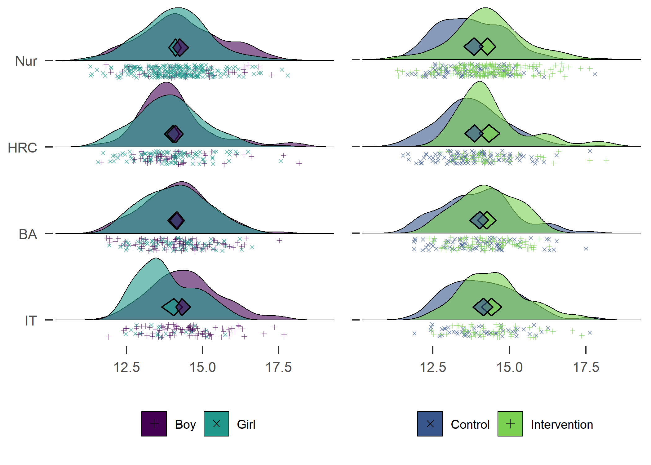
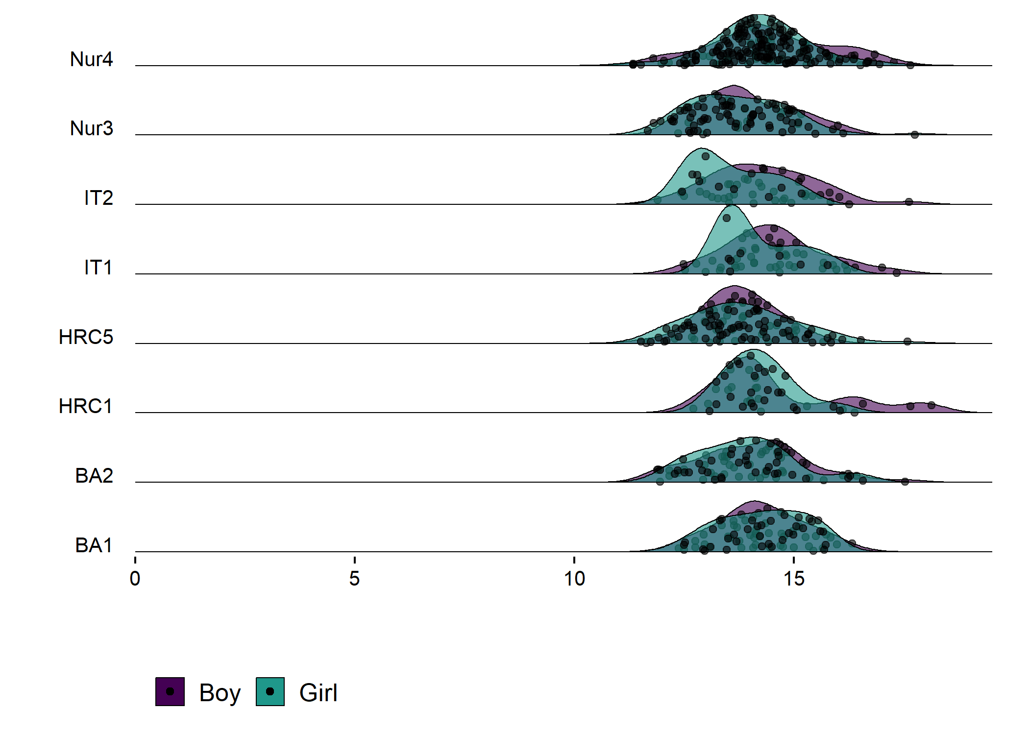
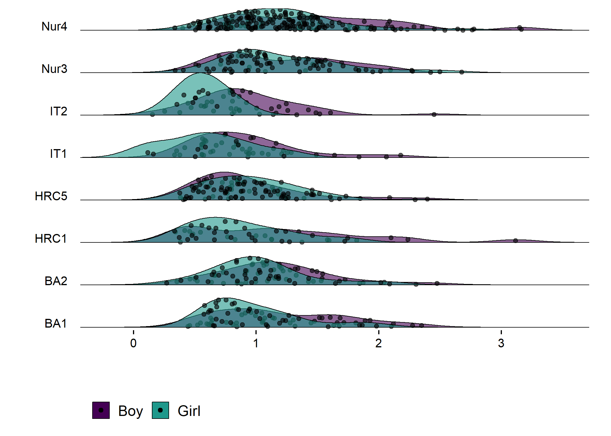
Accelerometer wear time. Nur = Practical nurse, HRC = Hotel, restaurant and catering, BA = Business and administration, IT = Information and communications technology.

Accelerometer wear time. Nur = Practical nurse, HRC = Hotel, restaurant and catering, BA = Business and administration, IT = Information and communications technology.

Accelerometer-measured MVPA

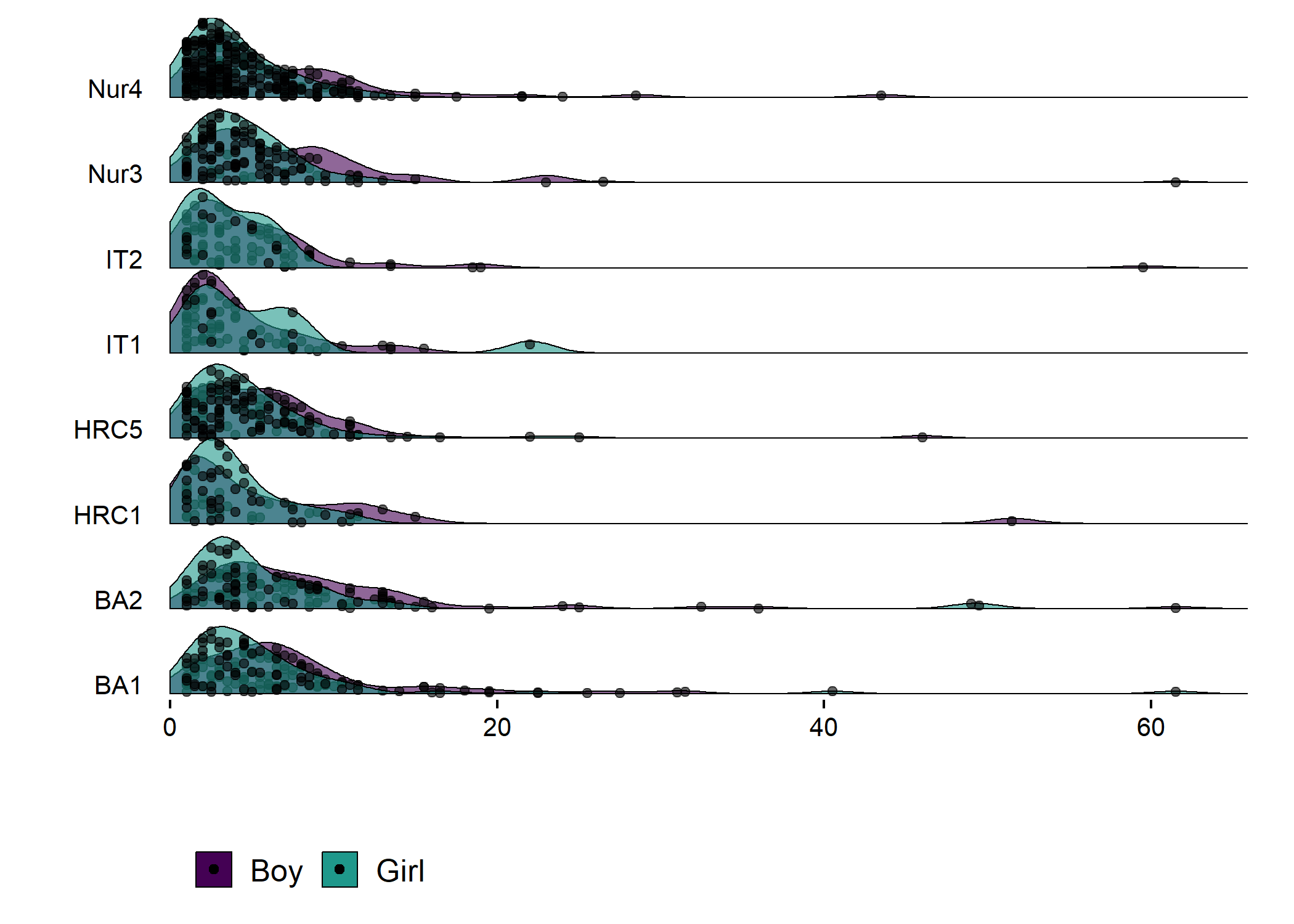
Contrary to some other findings, in our sample girls were more active than boys.

\(~\) \(~\)

Density plot by intervention and gender


# Create data frame
densplot <- d
levels(densplot$intervention) <- c("Control", "Intervention")
levels(densplot$girl) <- recode(densplot$girl, "boy" = "Boys", "girl" = "Girls")

# This gives side-by-side plots. There's a third plot below the two, which is fake to include x-axis text.
layout(matrix(c(1, 2, 3, 3), nrow = 2, ncol = 2, byrow = TRUE),
       widths = c(0.5, 0.5), heights = c(0.45, 0.05))

# Minimise whitespace; see https://stackoverflow.com/questions/15848942/how-to-reduce-space-gap-between-multiple-graphs-in-r
par(mai = c(0.3, 0.3, 0.1, 0.0)) 

## Girls vs. boys
# Choose only the variables needed and drop NA
dens <- densplot %>% dplyr::select(mvpaAccelerometer_T1, girl) %>% 
  dplyr::filter(complete.cases(.))

# Set random number generator for reproducibility of bootstrap test of equal densities
set.seed(10)

# Make plot
sm.mvpaAccelerometer_T1_2 <- sm.density.compare2(as.numeric(dens$mvpaAccelerometer_T1), 
                                               as.factor(dens$girl), 
                                               model = "equal",
                                               xlab = "", ylab = "",
                                               col = viridis::viridis(4, end  =  0.8)[c(3, 1)], 
                                               lty = c(1,3), yaxt = "n",
                                               bandcol = 'LightGray', 
                                               lwd = (c(2,2)))
## 
## Test of equal densities:  p-value =  0.12
legend("topright", levels(dens$girl), col = viridis::viridis(4, end = 0.8)[c(1, 3)], lty = c(3,1), lwd = (c(2,2)))
mtext(side = 2, "Density", line = 0.5)

## Intervention vs. control
# Choose only the variables needed and drop NA
dens <- densplot %>% dplyr::select(mvpaAccelerometer_T1, intervention) %>% 
  dplyr::filter(complete.cases(.))

# Set random number generator for reproducibility of bootstrap test of equal densities
set.seed(10)
# Make plot
sm.mvpaAccelerometer_T1_2 <- sm.density.compare2(as.numeric(dens$mvpaAccelerometer_T1), 
                                               as.factor(dens$intervention), 
                                               model = "equal", 
                                               xlab = "", ylab = "",
                                               col = viridis::viridis(4, end = 0.8)[c(2, 4)], 
                                               lty = c(3,1), yaxt = "n",
                                               bandcol = 'LightGray', 
                                               lwd = (c(2,2)))
## 
## Test of equal densities:  p-value =  0.14
legend("topright", levels(dens$intervention), col = viridis::viridis(4, end = 0.8)[c(2, 4)], lty=c(3,1), lwd=(c(2,2)))

# Create x-axis label. See https://stackoverflow.com/questions/11198767/how-to-annotate-across-or-between-plots-in-multi-plot-panels-in-r
par(mar = c(0,0,0,0)) 
plot(1, 1, type = "n", frame.plot = FALSE, axes = FALSE) # Fake plot for x-axis label
text(x = 1.02, y = 1.3, labels = "MVPA hours", pos = 1)
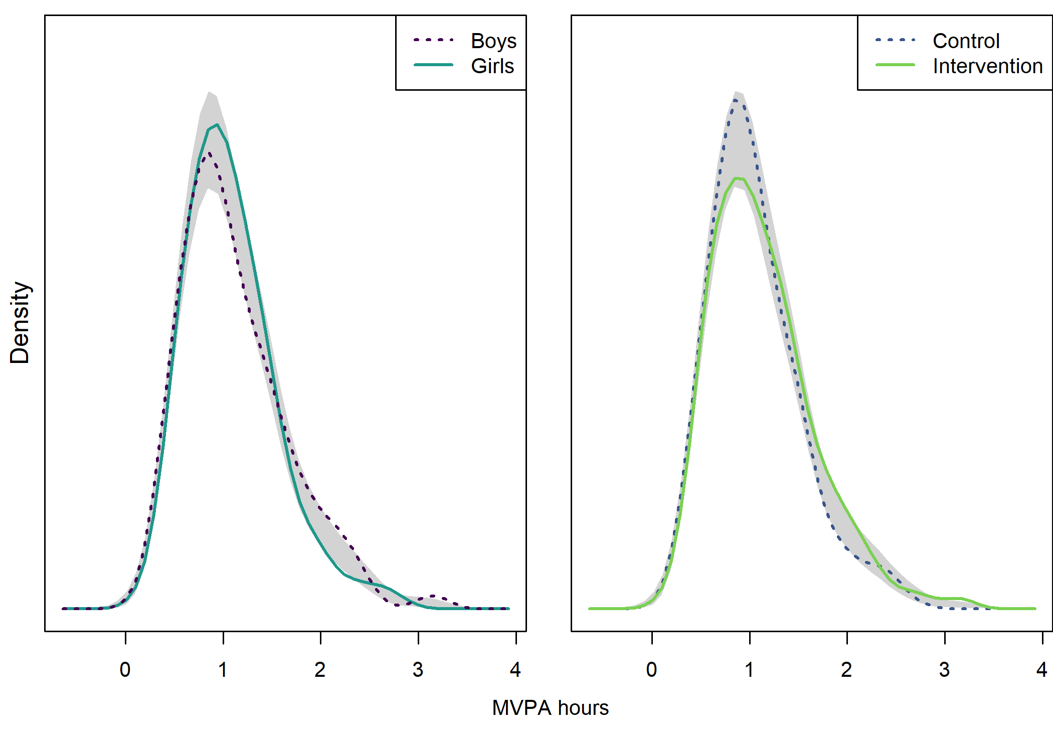
Data preparation

Description

The tab “Information on data preparation” of this section present information on data preparation for the plot \(~\) \(~\)

Information on data preparation

Prepare data

# m_mvpaAccelerometer_trackgirl <- brms::bf(mvpaAccelerometer_T1 ~ (1 | track:girl)) %>% 
#   brms::brm(., data = df, chains = 4, iter = 4000, control = list(adapt_delta = 0.95))
# 
# brms::prior_summary(m_mvpaAccelerometer_trackgirl, data = df)
# 
# m_mvpaAccelerometer_trackgirl
# 
# b_intercept <- brms::fixef(m_mvpaAccelerometer_trackgirl)[1]
# 
# # This gives estimates only:
# PA_trackgirl_estimates <- brms::ranef(m_mvpaAccelerometer_trackgirl)[[1]][1:10]
# 
# # The 2.5%ile:
# PA_trackgirl_CIL <- brms::ranef(m_mvpaAccelerometer_trackgirl)[[1]][21:30]
# 
# # The 97.5%ile:
# PA_trackgirl_CIH <- brms::ranef(m_mvpaAccelerometer_trackgirl)[[1]][31:40]
# 
# PA_trackgirl_ci <- data.frame(PA_trackgirl_CIL, PA_trackgirl_estimates, PA_trackgirl_CIH, Variable = labels(brms::ranef(m_mvpaAccelerometer_trackgirl))) %>% 
#   dplyr::mutate(b_intercept = rep(b_intercept, 10)) %>% 
#   dplyr::mutate(PA_trackgirl_CIL = PA_trackgirl_CIL + b_intercept,
#          PA_trackgirl_estimates = PA_trackgirl_estimates + b_intercept,
#          PA_trackgirl_CIH = PA_trackgirl_CIH + b_intercept,
#          track = c('BA_boy',
#                    'BA_girl',
#                    'HRC_boy',
#                    'HRC_girl',
#                    'IT_boy',
#                    'IT_girl',
#                    'Nur_boy',
#                    'Nur_girl',
#                    'Other_boy',
#                    'Other_girl'
# ))
# 
# PA_trackgirl_diamonds_girl <- rbind(
# PA_trackgirl_ci %>% dplyr::filter(track == "Nur_girl"),
# PA_trackgirl_ci %>% dplyr::filter(track == "HRC_girl"),
# PA_trackgirl_ci %>% dplyr::filter(track == "BA_girl"),
# PA_trackgirl_ci %>% dplyr::filter(track == "IT_girl")) %>% 
#   arrange(-row_number()) # reverse order of rows to make them right for the plot to come
# 
# PA_trackgirl_diamonds_boy <- rbind(
# PA_trackgirl_ci %>% dplyr::filter(track == "Nur_boy"),
# PA_trackgirl_ci %>% dplyr::filter(track == "HRC_boy"),
# PA_trackgirl_ci %>% dplyr::filter(track == "BA_boy"),
# PA_trackgirl_ci %>% dplyr::filter(track == "IT_boy")) %>% 
#   arrange(-row_number()) # reverse order of rows to make them right for the plot to come
# 
# 
# m_mvpaAccelerometer_trackintervention <- brms::bf(mvpaAccelerometer_T1 ~ (1 | track:intervention)) %>% 
#   brms::brm(., data = df, chains = 4, iter = 4000, control = list(adapt_delta = 0.95))
# 
# brms::prior_summary(m_mvpaAccelerometer_trackintervention, data = df)
# 
# m_mvpaAccelerometer_trackintervention
# 
# b_intercept <- brms::fixef(m_mvpaAccelerometer_trackintervention)[1]
# 
# # This gives estimates only:
# PA_trackintervention_estimates <- brms::ranef(m_mvpaAccelerometer_trackintervention)[[1]][1:10]
# 
# 
# # The 2.5%ile:
# PA_trackintervention_CIL <- brms::ranef(m_mvpaAccelerometer_trackintervention)[[1]][21:30]
# 
# # The 97.5%ile:
# PA_trackintervention_CIH <- brms::ranef(m_mvpaAccelerometer_trackintervention)[[1]][31:40]
# 
# PA_trackintervention_ci <- data.frame(PA_trackintervention_CIL, PA_trackintervention_estimates, PA_trackintervention_CIH, Variable = labels(brms::ranef(m_mvpaAccelerometer_trackintervention))) %>% 
#   dplyr::mutate(b_intercept = rep(b_intercept, 10)) %>% 
#   dplyr::mutate(PA_trackintervention_CIL = PA_trackintervention_CIL + b_intercept,
#          PA_trackintervention_estimates = PA_trackintervention_estimates + b_intercept,
#          PA_trackintervention_CIH = PA_trackintervention_CIH + b_intercept,
#          track = c('BA_control',
#                    'BA_intervention',
#                    'HRC_control',
#                    'HRC_intervention',
#                    'IT_control',
#                    'IT_intervention',
#                    'Nur_control',
#                    'Nur_intervention',
#                    'Other_control',
#                    'Other_intervention'
# ))
# 
# PA_trackintervention_diamonds_intervention <- rbind(
# PA_trackintervention_ci %>% dplyr::filter(track == "Nur_intervention"),
# PA_trackintervention_ci %>% dplyr::filter(track == "HRC_intervention"),
# PA_trackintervention_ci %>% dplyr::filter(track == "BA_intervention"),
# PA_trackintervention_ci %>% dplyr::filter(track == "IT_intervention")) %>% 
#   arrange(-row_number()) # reverse order of rows to make them right for the plot to come
# 
# PA_trackintervention_diamonds_control <- rbind(
# PA_trackintervention_ci %>% dplyr::filter(track == "Nur_control"),
# PA_trackintervention_ci %>% dplyr::filter(track == "HRC_control"),
# PA_trackintervention_ci %>% dplyr::filter(track == "BA_control"),
# PA_trackintervention_ci %>% dplyr::filter(track == "IT_control")) %>% 
#   arrange(-row_number()) # reverse order of rows to make them right for the plot to come
# 
# # readr::write_rds(PA_trackgirl_diamonds_girl, 
# #                  path = "./Rdata_files/PA_trackgirl_diamonds_girl.RDS")
# # readr::write_rds(PA_trackgirl_diamonds_boy, 
# #                  path = "./Rdata_files/PA_trackgirl_diamonds_boy.RDS")
# # readr::write_rds(PA_trackintervention_diamonds_intervention, 
# #                  path = "./Rdata_files/PA_trackintervention_diamonds_intervention.RDS")
# # readr::write_rds(PA_trackintervention_diamonds_control, 
# #                  path = "./Rdata_files/PA_trackintervention_diamonds_control.RDS")
# 
# save(PA_trackgirl_diamonds_girl, file = "./Rdata_files/PA_trackgirl_diamonds_girl.Rdata")
# save(PA_trackgirl_diamonds_boy, file = "./Rdata_files/PA_trackgirl_diamonds_boy.Rdata")
# save(PA_trackintervention_diamonds_intervention, file = "./Rdata_files/PA_trackintervention_diamonds_intervention.Rdata")
# save(PA_trackintervention_diamonds_control, file = "./Rdata_files/PA_trackintervention_diamonds_control.Rdata")

load("./Rdata_files/PA_trackgirl_diamonds_girl.Rdata")
load("./Rdata_files/PA_trackgirl_diamonds_boy.Rdata")
load("./Rdata_files/PA_trackintervention_diamonds_intervention.Rdata")
load("./Rdata_files/PA_trackintervention_diamonds_control.Rdata")

PA_trackgirl_diamonds_girl

Sensitivity analyses and robustness checks

Ideally, one would perform sensitivity analyses and robustness checks; e.g. comparing the estimates with frequentist multilevel models and following the WAMBS-checklist. Due to resource constraints, we are forced to forego this phase of analysis and instead, only show the linear model results for intercepts in each intervention-gender-track combination separately.


# To test the code with a single variable:
df_for_models_nested <- df %>% 
  dplyr::select(track, mvpaAccelerometer_T1, girl, intervention) %>% 
  dplyr::mutate(track = forcats::fct_recode(track, NULL = "Other")) %>%
  na.omit() %>% 
  dplyr::group_by(girl, intervention, track) %>% 
  tidyr::nest()

# This produced a data frame with columns "girl", "intervention", "track" and "data", the last of which is a data frame in each cell. E.g. for row wit intervention group girls in IT, there's a data frame for their values in the last column.

df_fitted <- df_for_models_nested %>% 
  dplyr::mutate(fit = map(data, ~ lm(mvpaAccelerometer_T1 ~ 1, data = .x)))
# Now there's a linear model for each combination in the data frame

df_fitted <- df_fitted %>% 
  dplyr::mutate(
    mean = map_dbl(fit, ~ coef(.x)[["(Intercept)"]]),
    ci_low = map_dbl(fit, ~ confint(.x)["(Intercept)", 1]),
    ci_high = map_dbl(fit, ~ confint(.x)["(Intercept)", 2]),
    nonmissings = map_dbl(fit, ~ nobs(.x))
  ) %>% 
  dplyr::mutate(mean = round(mean, 2),
         ci_low = round(ci_low, 2),
         ci_high = round(ci_high, 2))


## (here was an earlier attempt for random effects)
# df_fitted <- df_fitted %>% 
#   dplyr::mutate(
#     mean = map_dbl(fit, ~ lme4::fixef(.x)),
#     m_p = map(fit, ~ profile(.x)),
#     ci_low = map_dbl(m_p, ~ confint(.x)["(Intercept)", 1]),
#     ci_high = map_dbl(m_p, ~ confint(.x)["(Intercept)", 2]),
#     nonmissings = map_dbl(fit, ~ length(.x@resp$y))
#   )

## (here was was an earlier attempt to use sandwich estimator 
# df_for_sandwich_nested_withClusters <- df_for_sandwich_nested %>% 
#   dplyr::mutate(sandwich_clusters = purrr::map(data, magrittr::extract, c("group", "school", "track")))
# The last line selected the cluster variables from the data frame of each intervention-gender combination)

DT::datatable(df_fitted)

Density plot of girls and boys in different educational tracks and schools

Density plot by track


plot1 <- df %>% dplyr::select(id,
                              track = track,
                              girl,
                              PA = mvpaAccelerometer_T1)  %>%
  dplyr::filter(!is.na(track), track != "Other") %>% # Drop category "Other"
  dplyr::mutate(track = factor(track, levels = c("IT", "BA", "HRC", "Nur")),
                track = recode_factor(track, "IT" = "IT", "BA" = "BA", 
                                      "HRC" = "HRC", "Nur" = "Nur")) %>% 
  ggplot2::ggplot(aes(y = track)) +
  ggridges::geom_density_ridges2(aes(x = PA, colour = "black", 
                                    fill = paste(track, girl),
                                    point_color = girl,
                                    point_fill = girl,
                                    point_shape = girl),
                                  scale = .75, alpha = 0.6, size = 0.25,
                                  position = position_raincloud(width = 0.05, height = 0.15),
                                  # from = 0, to = 450,
                                  jittered_points = TRUE,
                                  point_size = 1) +
  labs(x = NULL,
       y = NULL) +
  scale_y_discrete(expand = c(0.1, 0)) +
  scale_x_continuous(expand = c(0.01, 0)) +
  ggridges::scale_fill_cyclical(
                                labels = c('BA boy' = "Boy", 'BA girl' = "Girl"),
                                values = viridis::viridis(4, end = 0.8)[c(1, 3)],
                                name = "", 
                                guide = guide_legend(override.aes = list(alpha = 1, 
                                                                         point_shape = c(3, 4),
                                                                         point_size = 2))) +
  ggridges::scale_colour_cyclical(values = "black") +
  ggridges::theme_ridges(grid = FALSE) +
  # ggplot2::scale_fill_manual(values = c("#A0FFA0", "#A0A0FF")) +
  ggridges::scale_discrete_manual(aesthetics = "point_color", 
                                  values = viridis::viridis(4, end = 0.8)[c(3, 1)],
                                  guide = "none") +
  ggridges::scale_discrete_manual(aesthetics = "point_fill",
                                  values = viridis::viridis(4, end = 0.8)[c(3, 1)],
                                  guide = "none") +
  ggridges::scale_discrete_manual(aesthetics = "point_shape", 
                                  values = c(4, 3),
                                  guide = "none") +
  papaja::theme_apa() +
  theme(legend.position = "bottom")

PA_trackgirl_diamonds_girl_hours <- PA_trackgirl_diamonds_girl %>% 
  dplyr::mutate_if(is.numeric, ~./60)
PA_trackgirl_diamonds_boy_hours <- PA_trackgirl_diamonds_boy %>% 
  dplyr::mutate_if(is.numeric, ~./60)

plot1 <- plot1 + 
  userfriendlyscience::diamondPlot(PA_trackgirl_diamonds_girl_hours, 
                                   returnLayerOnly = TRUE, 
                                   lineColor = "black", 
                                   color=viridis::viridis(4, end = 0.8)[3],
                                   alpha=.6, 
                                   fixedSize = 0.1, 
                                   otherAxisCol = (1:4 + .15)) + # specify y-position; option to move the diamond 
  userfriendlyscience::diamondPlot(PA_trackgirl_diamonds_boy_hours, 
                                   returnLayerOnly = TRUE, 
                                   lineColor = "black", 
                                   linetype = "solid", 
                                   color=viridis::viridis(4, end = 0.8)[1],
                                   alpha=.6, 
                                   fixedSize = 0.1, 
                                   otherAxisCol = (1:4 + .15))

# Draw plot with intervention and control densities

plot2 <- df %>% dplyr::select(id,
                              track = track,
                              intervention,
                              PA = mvpaAccelerometer_T1)  %>%
  dplyr::filter(!is.na(track), track != "Other") %>% # Drop category "Other"
  dplyr::mutate(track = factor(track, levels = c("IT", "BA", "HRC", "Nur")),
                track = recode_factor(track, "IT" = "IT", "BA" = "BA", 
                                      "HRC" = "HRC", "Nur" = "Nur")) %>% 
  ggplot2::ggplot(aes(y = track)) +
  ggridges::geom_density_ridges2(aes(x = PA, colour = "black", 
                                    fill = paste(track, intervention),
                                    point_color = intervention,
                                    point_fill = intervention,
                                    point_shape = intervention),
                                  scale = .75, alpha = 0.6, size = 0.25,
                                  position = position_raincloud(width = 0.05, height = 0.15),
                                  # from = 0, to = 450,
                                  jittered_points = TRUE,
                                  point_size = 1) +
  labs(x = NULL,
       y = NULL) +
  scale_y_discrete(expand = c(0.1, 0), labels = NULL) +
  scale_x_continuous(expand = c(0.01, 0)) +
  ggridges::scale_fill_cyclical(
                                labels = c('BA 0' = "Control", 'BA 1' = "Intervention"),
                                values = viridis::viridis(4, end = 0.8)[c(2, 4)],
                                name = "", 
                                guide = guide_legend(override.aes = list(alpha = 1, 
                                                                         point_shape = c(4, 3),
                                                                         point_size = 2))) +
  ggridges::scale_colour_cyclical(values = "black") +
  ggridges::theme_ridges(grid = FALSE) +
  # ggplot2::scale_fill_manual(values = c("#A0FFA0", "#A0A0FF")) +
  ggridges::scale_discrete_manual(aesthetics = "point_color", 
                                  values = viridis::viridis(4, end = 0.8)[c(2, 4)],
                                  guide = "none") +
  ggridges::scale_discrete_manual(aesthetics = "point_fill",
                                  values = viridis::viridis(4, end = 0.8)[c(2, 4)],
                                  guide = "none") +
  ggridges::scale_discrete_manual(aesthetics = "point_shape", 
                                  values = c(4, 3),
                                  guide = "none") +
  papaja::theme_apa() +
  theme(legend.position = "bottom")

PA_trackintervention_diamonds_intervention_hours <- PA_trackintervention_diamonds_intervention %>% 
  dplyr::mutate_if(is.numeric, ~./60)
PA_trackintervention_diamonds_control_hours <- PA_trackintervention_diamonds_control %>% 
  dplyr::mutate_if(is.numeric, ~./60)

plot2 <- plot2 + 
  userfriendlyscience::diamondPlot(PA_trackintervention_diamonds_intervention_hours, 
                                   returnLayerOnly = TRUE, 
                                   lineColor = "black",  
                                   color=viridis::viridis(4, end = 0.8)[4],
                                   alpha=.6, 
                                   fixedSize = 0.1, 
                                   otherAxisCol = (1:4 + .15)) +
  userfriendlyscience::diamondPlot(PA_trackintervention_diamonds_control_hours, 
                                   returnLayerOnly = TRUE, 
                                   lineColor = "black",  
                                   color=viridis::viridis(4, end = 0.8)[2],
                                   alpha=.6, 
                                   fixedSize = 0.1, 
                                   otherAxisCol = (1:4 + .15))

plot1 + plot2
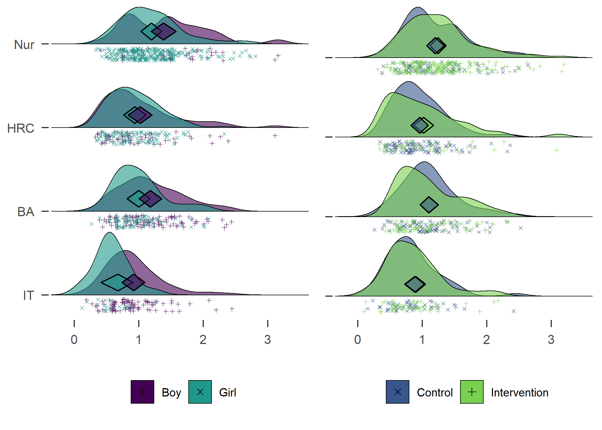
Accelerometer-measured MVPA. Nur = Practical nurse, HRC = Hotel, restaurant and catering, BA = Business and administration, IT = Information and communications technology.

Accelerometer-measured MVPA. Nur = Practical nurse, HRC = Hotel, restaurant and catering, BA = Business and administration, IT = Information and communications technology.

Self-reported MVPA days, previous week

Description

This section reports the question on how many days the participants did MVPA during the previous week. Question was formulated as “During the last 7 days, on how many days were you physically active so, that the activity was at least moderately vigorous, and at least 30 minutes of activity was accumulated during the day? Choose the correct option”.The scale allowed discrete values from zero to seven.

Data preparation

Description

The tab “Information on data preparation” of this section present information on data preparation for the plot

Information on data preparation

Code chunk below prepares data.

# m_padaysLastweek_trackgirl <- brms::bf(padaysLastweek_T1 ~ (1 | track:girl)) %>%
#   brms::brm(., data = df, chains = 4, iter = 4000, control = list(adapt_delta = 0.95))
# 
# brms::prior_summary(m_padaysLastweek_trackgirl, data = df)
# 
# m_padaysLastweek_trackgirl
# 
# b_intercept <- brms::fixef(m_padaysLastweek_trackgirl)[1]
# 
# # This gives estimates only:
# padaysLastweek_trackgirl_estimates <- brms::ranef(m_padaysLastweek_trackgirl)[[1]][1:10]
# 
# # The 2.5%ile:
# padaysLastweek_trackgirl_CIL <- brms::ranef(m_padaysLastweek_trackgirl)[[1]][21:30]
# 
# # The 97.5%ile:
# padaysLastweek_trackgirl_CIH <- brms::ranef(m_padaysLastweek_trackgirl)[[1]][31:40]
# 
# padaysLastweek_trackgirl_ci <- data.frame(padaysLastweek_trackgirl_CIL, padaysLastweek_trackgirl_estimates, padaysLastweek_trackgirl_CIH, Variable = labels(brms::ranef(m_padaysLastweek_trackgirl))) %>%
#   dplyr::mutate(b_intercept = rep(b_intercept, 10)) %>%
#   dplyr::mutate(padaysLastweek_trackgirl_CIL = padaysLastweek_trackgirl_CIL + b_intercept,
#          padaysLastweek_trackgirl_estimates = padaysLastweek_trackgirl_estimates + b_intercept,
#          padaysLastweek_trackgirl_CIH = padaysLastweek_trackgirl_CIH + b_intercept,
#          track = c('BA_boy',
#                    'BA_girl',
#                    'HRC_boy',
#                    'HRC_girl',
#                    'IT_boy',
#                    'IT_girl',
#                    'Nur_boy',
#                    'Nur_girl',
#                    'Other_boy',
#                    'Other_girl'
# ))
# 
# padaysLastweek_trackgirl_diamonds_girl <- rbind(
# padaysLastweek_trackgirl_ci %>% dplyr::filter(track == "Nur_girl"),
# padaysLastweek_trackgirl_ci %>% dplyr::filter(track == "HRC_girl"),
# padaysLastweek_trackgirl_ci %>% dplyr::filter(track == "BA_girl"),
# padaysLastweek_trackgirl_ci %>% dplyr::filter(track == "IT_girl")) %>%
#   arrange(-row_number()) # reverse order of rows to make them right for the plot to come
# 
# padaysLastweek_trackgirl_diamonds_boy <- rbind(
# padaysLastweek_trackgirl_ci %>% dplyr::filter(track == "Nur_boy"),
# padaysLastweek_trackgirl_ci %>% dplyr::filter(track == "HRC_boy"),
# padaysLastweek_trackgirl_ci %>% dplyr::filter(track == "BA_boy"),
# padaysLastweek_trackgirl_ci %>% dplyr::filter(track == "IT_boy")) %>%
#   arrange(-row_number()) # reverse order of rows to make them right for the plot to come
# 
# 
# m_padaysLastweek_trackintervention <- brms::bf(padaysLastweek_T1 ~ (1 | track:intervention)) %>%
#   brms::brm(., data = df, chains = 4, iter = 4000, control = list(adapt_delta = 0.95))
# 
# brms::prior_summary(m_padaysLastweek_trackintervention, data = df)
# 
# m_padaysLastweek_trackintervention
# 
# b_intercept <- brms::fixef(m_padaysLastweek_trackintervention)[1]
# 
# # This gives estimates only:
# padaysLastweek_trackintervention_estimates <- brms::ranef(m_padaysLastweek_trackintervention)[[1]][1:10]
# 
# # The 2.5%ile:
# padaysLastweek_trackintervention_CIL <- brms::ranef(m_padaysLastweek_trackintervention)[[1]][21:30]
# 
# # The 97.5%ile:
# padaysLastweek_trackintervention_CIH <- brms::ranef(m_padaysLastweek_trackintervention)[[1]][31:40]
# 
# padaysLastweek_trackintervention_ci <- data.frame(padaysLastweek_trackintervention_CIL, padaysLastweek_trackintervention_estimates, padaysLastweek_trackintervention_CIH, Variable = labels(brms::ranef(m_padaysLastweek_trackintervention))) %>%
#   dplyr::mutate(b_intercept = rep(b_intercept, 10)) %>%
#   dplyr::mutate(padaysLastweek_trackintervention_CIL = padaysLastweek_trackintervention_CIL + b_intercept,
#          padaysLastweek_trackintervention_estimates = padaysLastweek_trackintervention_estimates + b_intercept,
#          padaysLastweek_trackintervention_CIH = padaysLastweek_trackintervention_CIH + b_intercept,
#          track = c('BA_control',
#                    'BA_intervention',
#                    'HRC_control',
#                    'HRC_intervention',
#                    'IT_control',
#                    'IT_intervention',
#                    'Nur_control',
#                    'Nur_intervention',
#                    'Other_control',
#                    'Other_intervention'
# ))
# 
# padaysLastweek_trackintervention_diamonds_intervention <- rbind(
# padaysLastweek_trackintervention_ci %>% dplyr::filter(track == "Nur_intervention"),
# padaysLastweek_trackintervention_ci %>% dplyr::filter(track == "HRC_intervention"),
# padaysLastweek_trackintervention_ci %>% dplyr::filter(track == "BA_intervention"),
# padaysLastweek_trackintervention_ci %>% dplyr::filter(track == "IT_intervention")) %>%
#   arrange(-row_number()) # reverse order of rows to make them right for the plot to come
# 
# padaysLastweek_trackintervention_diamonds_control <- rbind(
# padaysLastweek_trackintervention_ci %>% dplyr::filter(track == "Nur_control"),
# padaysLastweek_trackintervention_ci %>% dplyr::filter(track == "HRC_control"),
# padaysLastweek_trackintervention_ci %>% dplyr::filter(track == "BA_control"),
# padaysLastweek_trackintervention_ci %>% dplyr::filter(track == "IT_control")) %>%
#   arrange(-row_number()) # reverse order of rows to make them right for the plot to come
# 
# save(padaysLastweek_trackgirl_diamonds_girl, file = "./Rdata_files/padaysLastweek_trackgirl_diamonds_girl.Rdata")
# save(padaysLastweek_trackgirl_diamonds_boy, file = "./Rdata_files/padaysLastweek_trackgirl_diamonds_boy.Rdata")
# save(padaysLastweek_trackintervention_diamonds_intervention, file = "./Rdata_files/padaysLastweek_trackintervention_diamonds_intervention.Rdata")
# save(padaysLastweek_trackintervention_diamonds_control, file = "./Rdata_files/padaysLastweek_trackintervention_diamonds_control.Rdata")

load("./Rdata_files/padaysLastweek_trackgirl_diamonds_girl.Rdata")
load("./Rdata_files/padaysLastweek_trackgirl_diamonds_boy.Rdata")
load("./Rdata_files/padaysLastweek_trackintervention_diamonds_intervention.Rdata")
load("./Rdata_files/padaysLastweek_trackintervention_diamonds_control.Rdata")

Density plot by intervention and gender


# Create data frame
densplot <- d
levels(densplot$intervention) <- c("Control", "Intervention")
levels(densplot$girl) <- recode(densplot$girl, "boy" = "Boys", "girl" = "Girls")

# This gives side-by-side plots. There's a third plot below the two, which is fake to include x-axis text.
layout(matrix(c(1, 2, 3, 3), nrow = 2, ncol = 2, byrow = TRUE),
       widths = c(0.5, 0.5), heights = c(0.45, 0.05))

# Minimise whitespace; see https://stackoverflow.com/questions/15848942/how-to-reduce-space-gap-between-multiple-graphs-in-r
par(mai = c(0.3, 0.3, 0.1, 0.0)) 

## Girls vs. boys
# Choose only the variables needed and drop NA
dens <- densplot %>% dplyr::select(padaysLastweek_T1, girl) %>% 
  dplyr::filter(complete.cases(.))

# Set random number generator for reproducibility of bootstrap test of equal densities
set.seed(10)

# Make plot
sm.padaysLastweek_T1_2 <- sm.density.compare2(as.numeric(dens$padaysLastweek_T1), 
                                               as.factor(dens$girl), 
                                               model = "equal",
                                               xlab = "", ylab = "",
                                               col = viridis::viridis(4, end  =  0.8)[c(3, 1)], 
                                               lty = c(1, 3), yaxt = "n",
                                               bandcol = 'LightGray', 
                                               lwd = c(2, 2),
                                               xlim = c(0, 7))
## 
## Test of equal densities:  p-value =  0
legend("topright", levels(dens$girl), col = viridis::viridis(4, end = 0.8)[c(1, 3)], lty = c(3,1), lwd = (c(2,2)))
mtext(side = 2, "Density", line = 0.5)

## Intervention vs. control
# Choose only the variables needed and drop NA
dens <- densplot %>% dplyr::select(padaysLastweek_T1, intervention) %>% 
  dplyr::filter(complete.cases(.))

# Set random number generator for reproducibility of bootstrap test of equal densities
set.seed(10)
# Make plot
sm.padaysLastweek_T1_2 <- sm.density.compare2(as.numeric(dens$padaysLastweek_T1), 
                                               as.factor(dens$intervention), 
                                               model = "equal", 
                                               xlab = "", ylab = "",
                                               col = viridis::viridis(4, end = 0.8)[c(2, 4)], 
                                               lty = c(3, 1), yaxt = "n",
                                               bandcol = 'LightGray', 
                                               lwd = c(2, 2),
                                               xlim = c(0, 7))
## 
## Test of equal densities:  p-value =  0.09
legend("topright", levels(dens$intervention), col = viridis::viridis(4, end = 0.8)[c(2, 4)], lty=c(3,1), lwd=(c(2,2)))

# Create x-axis label. See https://stackoverflow.com/questions/11198767/how-to-annotate-across-or-between-plots-in-multi-plot-panels-in-r
par(mar = c(0,0,0,0)) 
plot(1, 1, type = "n", frame.plot = FALSE, axes = FALSE) # Fake plot for x-axis label
text(x = 1.02, y = 1.3, labels = "Self-reported number of days with >30 MVPA min previous week", pos = 1)
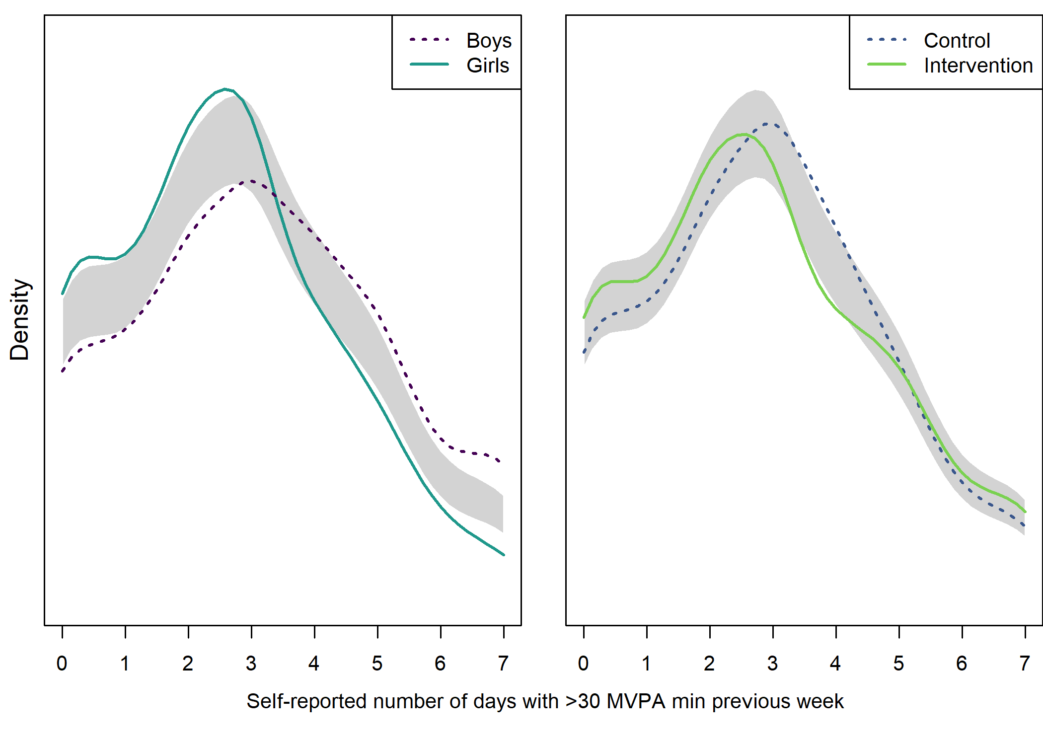
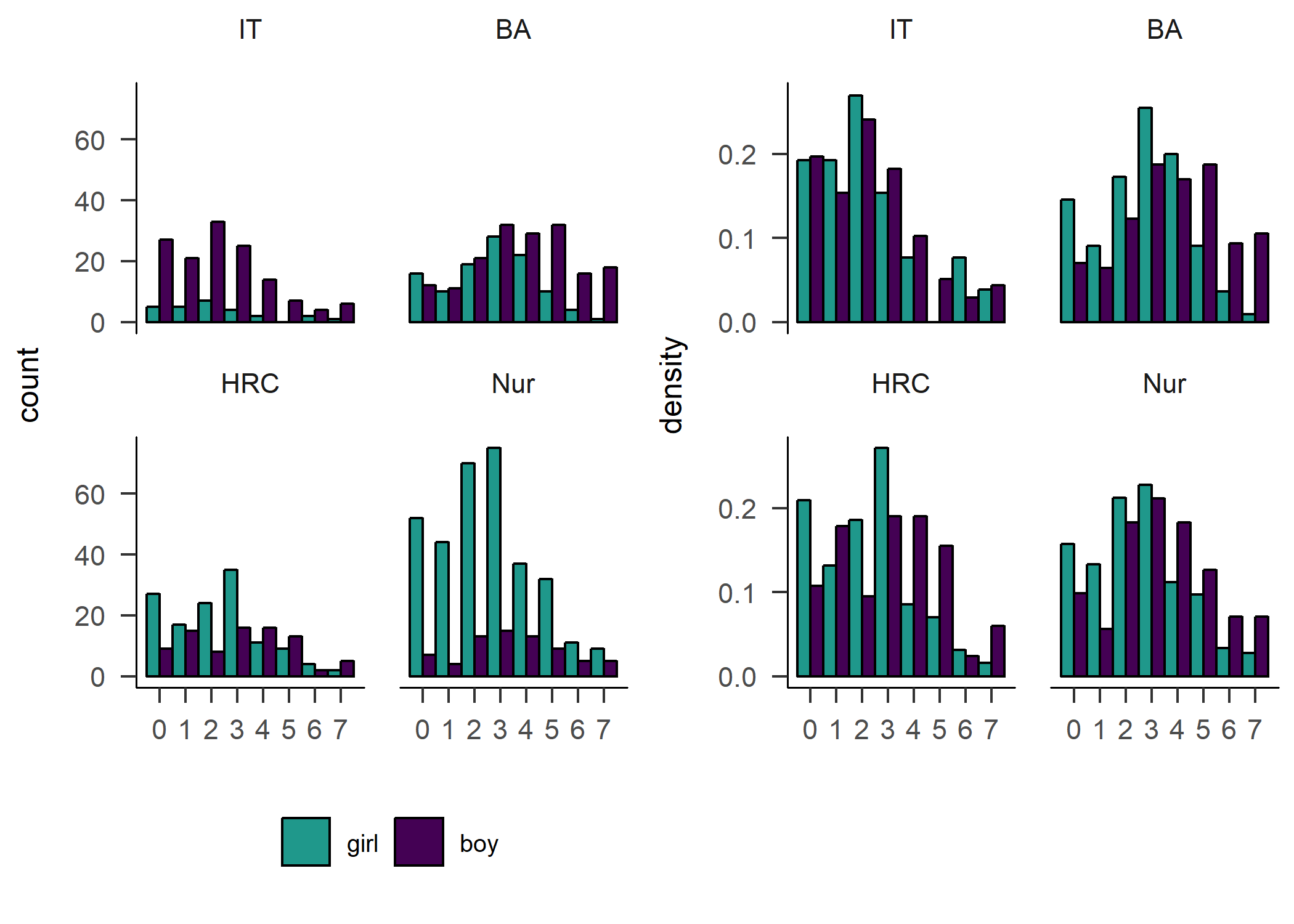
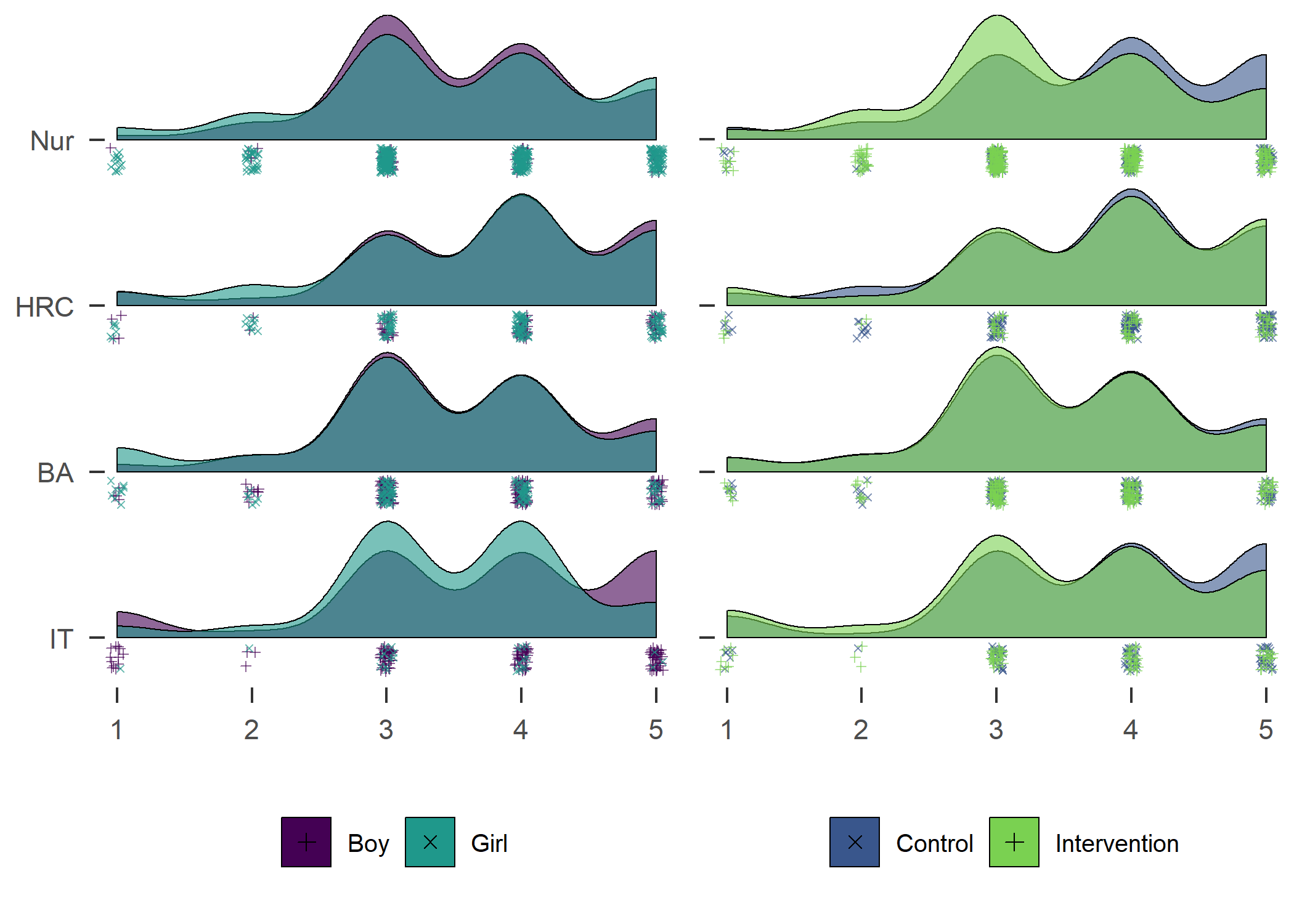
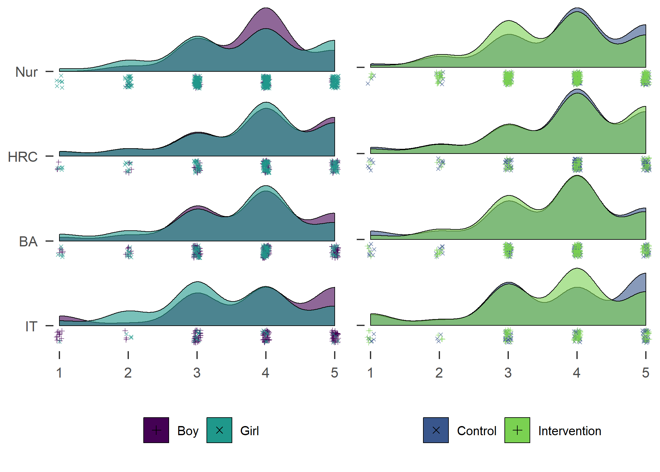
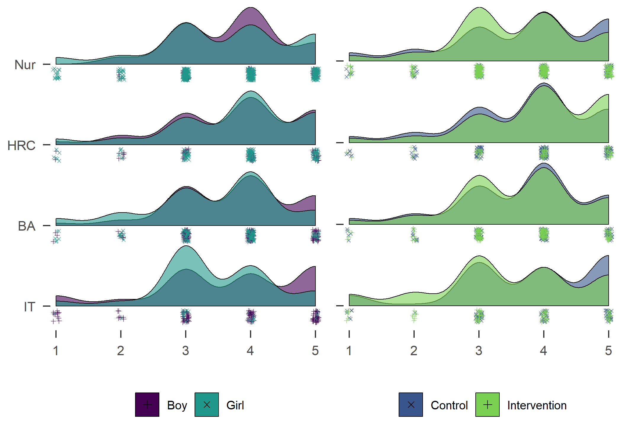
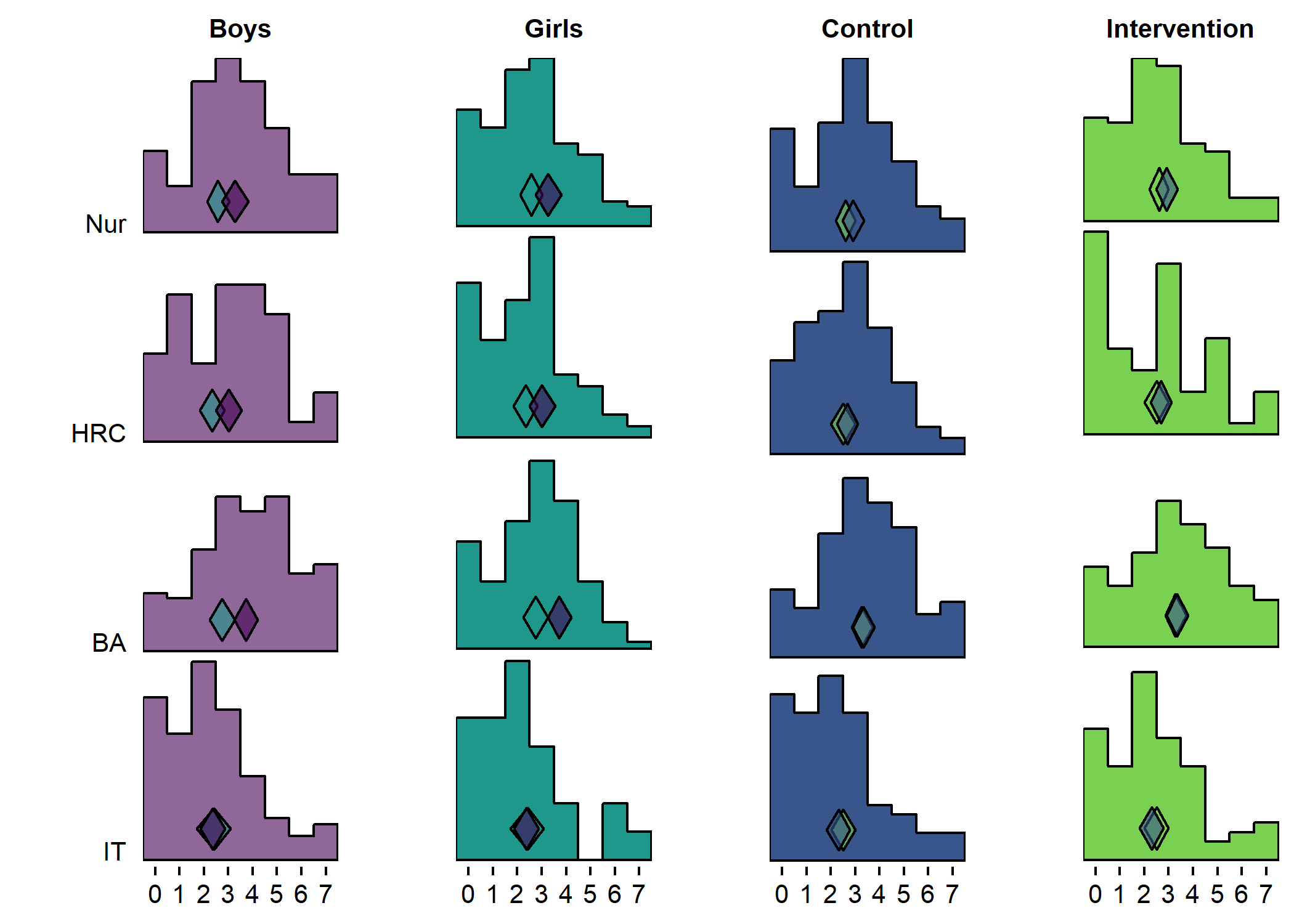
From the figure, we can see that there were more boys reporting a high number of MVPA days, and fewer boys reported low numbers. This effect was consistent among educational tracks. Boys and girls, as well as different educational tracks, differed largely in the types of PA they reported having engaged in during the previous month (see tab Tables and Estimators, at “Types of self-reported exercise”).

Density plot by track


plot1 <- df %>% dplyr::select(id,
                              track = track,
                              girl,
                              PA = padaysLastweek_T1)  %>%
  dplyr::filter(!is.na(track), track != "Other") %>% # Drop category "Other"
  dplyr::mutate(track = factor(track, levels = c("IT", "BA", "HRC", "Nur")),
                track = recode_factor(track, "IT" = "IT", "BA" = "BA", 
                                      "HRC" = "HRC", "Nur" = "Nur")) %>% 
  ggplot2::ggplot(aes(y = track)) +
  ggridges::geom_density_ridges2(aes(x = PA, colour = "black", 
                                    fill = paste(track, girl),
                                    point_color = girl,
                                    point_fill = girl,
                                    point_shape = girl),
                                  scale = .6, alpha = 0.6, size = 0.25,
                                  position = position_raincloud(width = 0.2, height = 0.4),
                                  # from = 0, to = 450,
                                  jittered_points = TRUE,
                                  point_size = 1,
                                  limits = c(0, 7)) +
  labs(x = NULL,
       y = NULL) +
  scale_y_discrete(expand = c(0.1, 0)) +
  scale_x_continuous(expand = c(0.01, 0), breaks = 0:7, limits = c(0, 7)) +
  ggridges::scale_fill_cyclical(
                                labels = c('BA boy' = "Boy", 'BA girl' = "Girl"),
                                values = viridis::viridis(4, end = 0.8)[c(1, 3)],
                                name = "", 
                                guide = guide_legend(override.aes = list(alpha = 1, 
                                                                         point_shape = c(3, 4),
                                                                         point_size = 2))) +
  ggridges::scale_colour_cyclical(values = "black") +
  ggridges::theme_ridges(grid = FALSE) +
  # ggplot2::scale_fill_manual(values = c("#A0FFA0", "#A0A0FF")) +
  ggridges::scale_discrete_manual(aesthetics = "point_color", 
                                  values = viridis::viridis(4, end = 0.8)[c(3, 1)],
                                  guide = "none") +
  ggridges::scale_discrete_manual(aesthetics = "point_fill",
                                  values = viridis::viridis(4, end = 0.8)[c(3, 1)],
                                  guide = "none") +
  ggridges::scale_discrete_manual(aesthetics = "point_shape", 
                                  values = c(4, 3),
                                  guide = "none") +
  papaja::theme_apa() +
  theme(legend.position = "bottom")

plot1 <- plot1 + 
  userfriendlyscience::diamondPlot(padaysLastweek_trackgirl_diamonds_girl, 
                                   returnLayerOnly = TRUE, 
                                   lineColor = "black", 
                                   color=viridis::viridis(4, end = 0.8)[3],
                                   alpha=.6, 
                                   fixedSize = 0.1, 
                                   otherAxisCol = (1:4 + .15)) + # specify y-position; option to move the diamond 
  userfriendlyscience::diamondPlot(padaysLastweek_trackgirl_diamonds_boy, 
                                   returnLayerOnly = TRUE, 
                                   lineColor = "black", 
                                   linetype = "solid", 
                                   color=viridis::viridis(4, end = 0.8)[1],
                                   alpha=.6, 
                                   fixedSize = 0.1, 
                                   otherAxisCol = (1:4 + .15))

# Draw plot with intervention and control densities

plot2 <- df %>% dplyr::select(id,
                              track = track,
                              intervention,
                              PA = padaysLastweek_T1)  %>%
  dplyr::filter(!is.na(track), track != "Other") %>% # Drop category "Other"
  dplyr::mutate(track = factor(track, levels = c("IT", "BA", "HRC", "Nur")),
                track = recode_factor(track, "IT" = "IT", "BA" = "BA", 
                                      "HRC" = "HRC", "Nur" = "Nur")) %>% 
  ggplot2::ggplot(aes(y = track)) +
  ggridges::geom_density_ridges2(aes(x = PA, colour = "black", 
                                    fill = paste(track, intervention),
                                    point_color = intervention,
                                    point_fill = intervention,
                                    point_shape = intervention),
                                  scale = .6, alpha = 0.6, size = 0.25,
                                  position = position_raincloud(width = 0.2, height = 0.4),
                                  # from = 0, to = 450,
                                  jittered_points = TRUE,
                                  point_size = 1,
                                  limits = c(0, 7)) +
  labs(x = NULL,
       y = NULL) +
  scale_y_discrete(expand = c(0.1, 0), labels = NULL) +
  scale_x_continuous(expand = c(0.01, 0), breaks = 0:7, limits = c(0, 7)) +
  ggridges::scale_fill_cyclical(
                                labels = c('BA 0' = "Control", 'BA 1' = "Intervention"),
                                values = viridis::viridis(4, end = 0.8)[c(2, 4)],
                                name = "", 
                                guide = guide_legend(override.aes = list(alpha = 1, 
                                                                         point_shape = c(4, 3),
                                                                         point_size = 2))) +
  ggridges::scale_colour_cyclical(values = "black") +
  ggridges::theme_ridges(grid = FALSE) +
  # ggplot2::scale_fill_manual(values = c("#A0FFA0", "#A0A0FF")) +
  ggridges::scale_discrete_manual(aesthetics = "point_color", 
                                  values = viridis::viridis(4, end = 0.8)[c(2, 4)],
                                  guide = "none") +
  ggridges::scale_discrete_manual(aesthetics = "point_fill",
                                  values = viridis::viridis(4, end = 0.8)[c(2, 4)],
                                  guide = "none") +
  ggridges::scale_discrete_manual(aesthetics = "point_shape", 
                                  values = c(4, 3),
                                  guide = "none") +
  papaja::theme_apa() +
  theme(legend.position = "bottom")

plot2 <- plot2 + 
  userfriendlyscience::diamondPlot(padaysLastweek_trackintervention_diamonds_intervention, 
                                   returnLayerOnly = TRUE, 
                                   lineColor = "black",  
                                   color=viridis::viridis(4, end = 0.8)[4],
                                   alpha=.6, 
                                   fixedSize = 0.1, 
                                   otherAxisCol = (1:4 + .15)) +
  userfriendlyscience::diamondPlot(padaysLastweek_trackintervention_diamonds_control, 
                                   returnLayerOnly = TRUE, 
                                   lineColor = "black",  
                                   color=viridis::viridis(4, end = 0.8)[2],
                                   alpha=.6, 
                                   fixedSize = 0.1, 
                                   otherAxisCol = (1:4 + .15))

plot1 + plot2
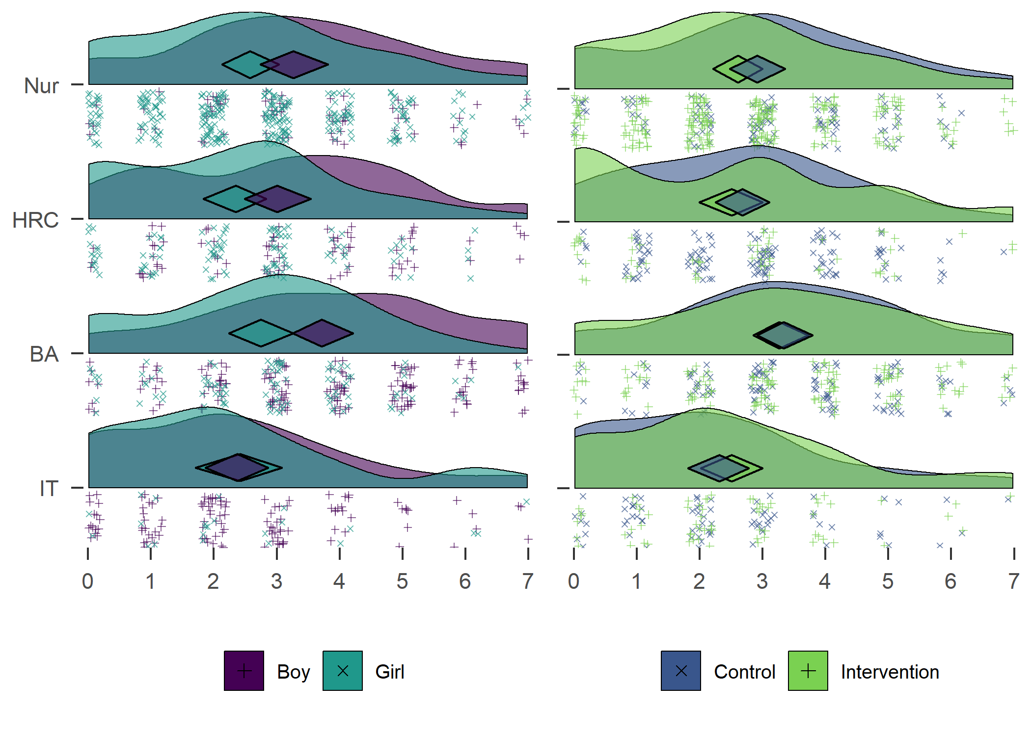
Self-reported number of days with > 30 MVPA min previous week. Nur = Practical nurse, HRC = Hotel, restaurant and catering, BA = Business and administration, IT = Information and communications technology.

Self-reported number of days with > 30 MVPA min previous week. Nur = Practical nurse, HRC = Hotel, restaurant and catering, BA = Business and administration, IT = Information and communications technology.

Histogram 1

plotboys <- df %>% dplyr::select(id,
                                 track = track,
                                 girl,
                                 padaysLastweek_T1)  %>%
  dplyr::filter(!is.na(track), track != "Other", girl == "boy") %>% # Drop category "Other"
  dplyr::mutate(track = factor(track, levels = c("IT", "BA", "HRC", "Nur")),
                track = recode_factor(track, "IT" = "IT", "BA" = "BA", 
                                      "HRC" = "HRC", "Nur" = "Nur")) %>% 
  ggplot2::ggplot(aes(y = track)) +
  ggridges::geom_density_ridges2(aes(x = padaysLastweek_T1, fill = girl), stat = "binline", binwidth = 1, scale = 0.95, alpha = 0.6) +
  scale_x_continuous(breaks = c(0:7), expand = c(0, 0), name = NULL) +
  scale_y_discrete(expand = c(0.01, 0), name = "") +
  ggridges::scale_fill_cyclical(values = viridis::viridis(4, end = 0.8)[1]) +
  labs(title = "Boys") +
  guides(y = "none") +
  ggridges::theme_ridges(grid = FALSE) +
  theme(axis.title.x = element_text(hjust = 0.5),
        axis.title.y = element_text(hjust = 0.5),
        plot.title = element_text(hjust = 0.5, size = 10),
        axis.text=element_text(size=10)) +
  coord_cartesian(xlim = c(-0.5, 7.5))

plotboys <- plotboys + 
  userfriendlyscience::diamondPlot(padaysLastweek_trackgirl_diamonds_girl, 
                                   returnLayerOnly = TRUE, 
                                   lineColor = "black", 
                                   color=viridis::viridis(4, end = 0.8)[3],
                                   alpha=.6, 
                                   fixedSize = 0.1, 
                                   otherAxisCol = (1:4 + .15)) + # specify y-position; option to move the diamond 
  userfriendlyscience::diamondPlot(padaysLastweek_trackgirl_diamonds_boy, 
                                   returnLayerOnly = TRUE, 
                                   lineColor = "black", 
                                   linetype = "solid", 
                                   color=viridis::viridis(4, end = 0.8)[1],
                                   alpha=.6, 
                                   fixedSize = 0.1, 
                                   otherAxisCol = (1:4 + .15))

plotgirls <- df %>% dplyr::select(id,
                                 track = track,
                                 girl,
                                 padaysLastweek_T1)  %>%
  dplyr::filter(!is.na(track), track != "Other", girl == "girl") %>% # Drop category "Other"
  dplyr::mutate(track = factor(track, levels = c("IT", "BA", "HRC", "Nur")),
                track = recode_factor(track, "IT" = "IT", "BA" = "BA", 
                                      "HRC" = "HRC", "Nur" = "Nur")) %>% 
  ggplot2::ggplot(aes(y = track)) +
  ggridges::geom_density_ridges2(aes(x = padaysLastweek_T1, fill = girl), stat = "binline", binwidth = 1, scale = 0.95) +
  scale_x_continuous(breaks = c(0:7), expand = c(0, 0), name = NULL) +
  scale_y_discrete(expand = c(0.01, 0), name = "", labels = NULL) +
  ggridges::scale_fill_cyclical(values = viridis::viridis(4, end = 0.8)[3]) +
  labs(title = "Girls") +
  guides(y = "none") +
  ggridges::theme_ridges(grid = FALSE) +
  theme(axis.title.x = element_text(hjust = 0.5),
        axis.title.y = element_text(hjust = 0.5),
        plot.title = element_text(hjust = 0.5, size = 10),
        axis.text=element_text(size=10)) +
  coord_cartesian(xlim = c(-0.5, 7.5))

plotgirls <- plotgirls + 
  userfriendlyscience::diamondPlot(padaysLastweek_trackgirl_diamonds_girl, 
                                   returnLayerOnly = TRUE, 
                                   lineColor = "black", 
                                   color=viridis::viridis(4, end = 0.8)[3],
                                   alpha=.6, 
                                   fixedSize = 0.1, 
                                   otherAxisCol = (1:4 + .15)) + # specify y-position; option to move the diamond 
  userfriendlyscience::diamondPlot(padaysLastweek_trackgirl_diamonds_boy, 
                                   returnLayerOnly = TRUE, 
                                   lineColor = "black", 
                                   linetype = "solid", 
                                   color=viridis::viridis(4, end = 0.8)[1],
                                   alpha=.6, 
                                   fixedSize = 0.1, 
                                   otherAxisCol = (1:4 + .15))


plotcontrol <- df %>% dplyr::select(id,
                                 track = track,
                                 intervention,
                                 padaysLastweek_T1)  %>%
  dplyr::filter(!is.na(track), track != "Other", intervention == "0") %>% # Drop category "Other"
  dplyr::mutate(track = factor(track, levels = c("IT", "BA", "HRC", "Nur")),
                track = recode_factor(track, "IT" = "IT", "BA" = "BA", 
                                      "HRC" = "HRC", "Nur" = "Nur")) %>% 
  ggplot2::ggplot(aes(y = track)) +
  ggridges::geom_density_ridges2(aes(x = padaysLastweek_T1, fill = intervention), stat = "binline", binwidth = 1, scale = 0.95) +
  scale_x_continuous(breaks = c(0:7), expand = c(0, 0), name = NULL) +
  scale_y_discrete(expand = c(0.01, 0), name = "", labels = NULL) +
  ggridges::scale_fill_cyclical(values = viridis::viridis(4, end = 0.8)[2]) +
  labs(title = "Control") +
  guides(y = "none") +
  ggridges::theme_ridges(grid = FALSE) +
  theme(axis.title.x = element_text(hjust = 0.5),
        axis.title.y = element_text(hjust = 0.5),
        plot.title = element_text(hjust = 0.5, size = 10),
        axis.text=element_text(size=10)) +
  coord_cartesian(xlim = c(-0.5, 7.5))

plotcontrol <- plotcontrol + 
  userfriendlyscience::diamondPlot(padaysLastweek_trackintervention_diamonds_intervention, 
                                   returnLayerOnly = TRUE, 
                                   lineColor = "black",  
                                   color=viridis::viridis(4, end = 0.8)[4],
                                   alpha=.6, 
                                   fixedSize = 0.1, 
                                   otherAxisCol = (1:4 + .15)) +
  userfriendlyscience::diamondPlot(padaysLastweek_trackintervention_diamonds_control, 
                                   returnLayerOnly = TRUE, 
                                   lineColor = "black",  
                                   color=viridis::viridis(4, end = 0.8)[2],
                                   alpha=.6, 
                                   fixedSize = 0.1, 
                                   otherAxisCol = (1:4 + .15))

plotintervention <- df %>% dplyr::select(id,
                                 track = track,
                                 intervention,
                                 padaysLastweek_T1)  %>%
  dplyr::filter(!is.na(track), track != "Other", intervention == "1") %>% # Drop category "Other"
  dplyr::mutate(track = factor(track, levels = c("IT", "BA", "HRC", "Nur")),
                track = recode_factor(track, "IT" = "IT", "BA" = "BA", 
                                      "HRC" = "HRC", "Nur" = "Nur")) %>% 
  ggplot2::ggplot(aes(y = track)) +
  ggridges::geom_density_ridges2(aes(x = padaysLastweek_T1, fill = intervention), stat = "binline", binwidth = 1, scale = 0.95) +
  scale_x_continuous(breaks = c(0:7), expand = c(0, 0), name = NULL) +
  scale_y_discrete(expand = c(0.01, 0), name = "", labels = NULL) +
  ggridges::scale_fill_cyclical(values = viridis::viridis(4, end = 0.8)[4]) +
  labs(title = "Intervention") +
  guides(y = "none") +
  ggridges::theme_ridges(grid = FALSE) +
  theme(axis.title.x = element_text(hjust = 0.5),
        axis.title.y = element_text(hjust = 0.5),
        plot.title = element_text(hjust = 0.5, size = 10),
        axis.text=element_text(size=10)) +
  coord_cartesian(xlim = c(-0.5, 7.5))

plotintervention <- plotintervention + 
  userfriendlyscience::diamondPlot(padaysLastweek_trackintervention_diamonds_intervention, 
                                   returnLayerOnly = TRUE, 
                                   lineColor = "black",  
                                   color=viridis::viridis(4, end = 0.8)[4],
                                   alpha=.6, 
                                   fixedSize = 0.1, 
                                   otherAxisCol = (1:4 + .15)) +
  userfriendlyscience::diamondPlot(padaysLastweek_trackintervention_diamonds_control, 
                                   returnLayerOnly = TRUE, 
                                   lineColor = "black",  
                                   color=viridis::viridis(4, end = 0.8)[2],
                                   alpha=.6, 
                                   fixedSize = 0.1, 
                                   otherAxisCol = (1:4 + .15))

plotboys + plotgirls + plotcontrol + plotintervention + plot_layout(ncol = 4)
Histogram 2


hist_padaysLastweek_intervention_count <- df %>% dplyr::select(id,
                                 track = track,
                                 intervention,
                                 padaysLastweek_T1)  %>%
  dplyr::filter(!is.na(track), track != "Other") %>% # Drop category "Other"
  dplyr::mutate(track = factor(track, levels = c("IT", "BA", "HRC", "Nur")),
                track = recode_factor(track, "IT" = "IT", "BA" = "BA", 
                                      "HRC" = "HRC", "Nur" = "Nur"),
                padaysLastweek_T1 = as.integer(padaysLastweek_T1)) %>% 
  ggplot(aes(x=padaysLastweek_T1, fill=intervention)) +
  geom_histogram(binwidth = 1, position = "dodge", color = "black") +
  scale_x_continuous(breaks = 0:7) +
  labs(x = NULL) + 
  scale_fill_manual(values = viridis::viridis(4, end = 0.8)[c(2, 4)], 
                    name = NULL, 
                    labels = c("0" = "control", "1" = "intervention")) +
  facet_wrap("track") + 
  theme(legend.position = "bottom")

hist_padaysLastweek_intervention_density <- df %>% dplyr::select(id,
                                 track = track,
                                 intervention,
                                 padaysLastweek_T1)  %>%
  dplyr::filter(!is.na(track), track != "Other") %>% # Drop category "Other"
  dplyr::mutate(track = factor(track, levels = c("IT", "BA", "HRC", "Nur")),
                track = recode_factor(track, "IT" = "IT", "BA" = "BA", 
                                      "HRC" = "HRC", "Nur" = "Nur"),
                padaysLastweek_T1 = as.integer(padaysLastweek_T1)) %>% 
  ggplot(aes(x=padaysLastweek_T1, y = ..density.., fill=intervention)) +
  geom_histogram(binwidth = 1, position = "dodge", color = "black") +
  scale_x_continuous(breaks = 0:7) +
  labs(x = NULL) + 
  scale_fill_manual(values = viridis::viridis(4, end = 0.8)[c(2, 4)], 
                    guide = FALSE) +
  facet_wrap("track")

hist_padaysLastweek_intervention_count + hist_padaysLastweek_intervention_density
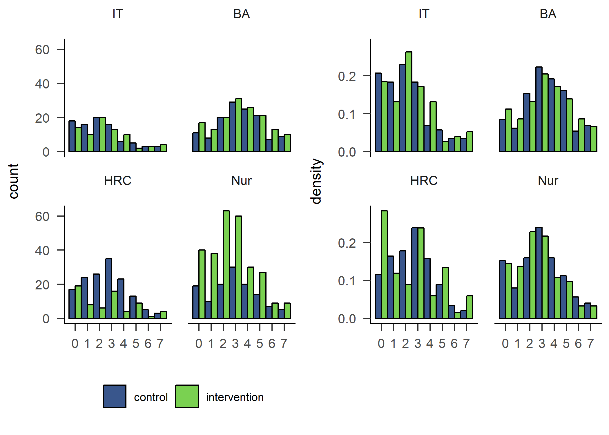
The number of days participants reported doing PA on, suggested a different picture of difference between genders in activity. Boys reported being more active in all but the IT track. The effect is also shown in the following variable on self-reported MVPA time.

Self-reported MVPA time

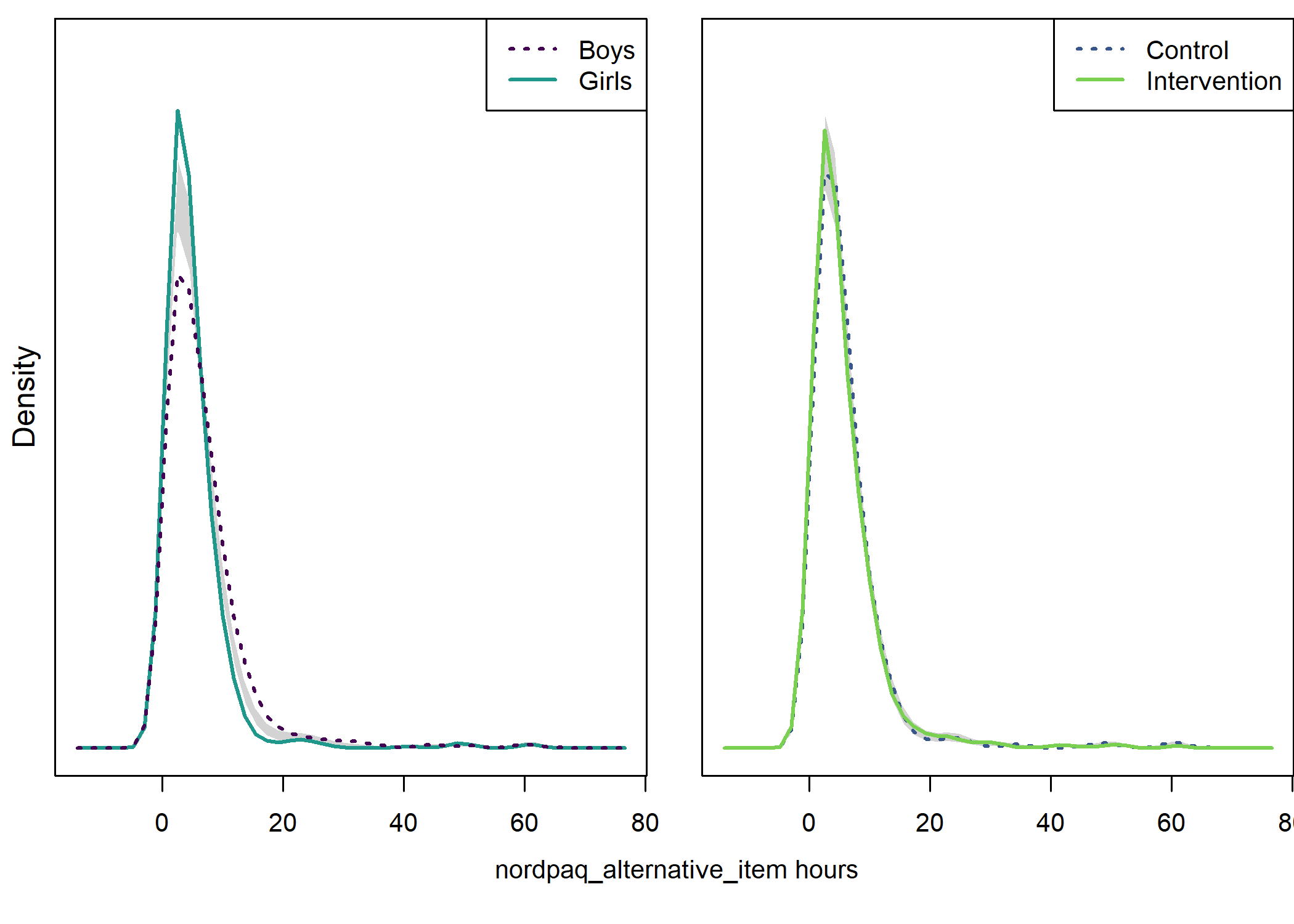
This question was “During the last 7 days, how many hours of the previously described [i.e. moderate-to-vigorous] physical activity was accumulated during your free time? Give your answer to the nearest 30 minutes.” The answer was given by inputing hours and minutes, the latter field allowing for either zero or 30 minutes to be inputed.

Density plot by intervention and gender


# Create data frame
densplot <- d
levels(densplot$intervention) <- c("Control", "Intervention")
levels(densplot$girl) <- recode(densplot$girl, "boy" = "Boys", "girl" = "Girls")

# This gives side-by-side plots. There's a third plot below the two, which is fake to include x-axis text.
layout(matrix(c(1, 2, 3, 3), nrow = 2, ncol = 2, byrow = TRUE),
       widths = c(0.5, 0.5), heights = c(0.45, 0.05))

# Minimise whitespace; see https://stackoverflow.com/questions/15848942/how-to-reduce-space-gap-between-multiple-graphs-in-r
par(mai = c(0.3, 0.3, 0.1, 0.0)) 

## Girls vs. boys
# Choose only the variables needed and drop NA
dens <- densplot %>% dplyr::select(leisuretimeMvpaHoursLastweek_T1, girl) %>% 
  dplyr::filter(complete.cases(.))

# Set random number generator for reproducibility of bootstrap test of equal densities
set.seed(10)

# Make plot
sm.leisuretimeMvpaHoursLastweek_T1_2 <- sm.density.compare2(as.numeric(dens$leisuretimeMvpaHoursLastweek_T1), 
                                               as.factor(dens$girl), 
                                               model = "equal",
                                               xlab = "", ylab = "",
                                               col = viridis::viridis(4, end  =  0.8)[c(3, 1)], 
                                               lty = c(1,3), yaxt = "n",
                                               bandcol = 'LightGray', 
                                               lwd = (c(2,2)))
## 
## Test of equal densities:  p-value =  0
legend("topright", levels(dens$girl), col = viridis::viridis(4, end = 0.8)[c(1, 3)], lty = c(3,1), lwd = (c(2,2)))
mtext(side = 2, "Density", line = 0.5)

## Intervention vs. control
# Choose only the variables needed and drop NA
dens <- densplot %>% dplyr::select(leisuretimeMvpaHoursLastweek_T1, intervention) %>% 
  dplyr::filter(complete.cases(.))

# Set random number generator for reproducibility of bootstrap test of equal densities
set.seed(10)
# Make plot
sm.leisuretimeMvpaHoursLastweek_T1_2 <- sm.density.compare2(as.numeric(dens$leisuretimeMvpaHoursLastweek_T1), 
                                               as.factor(dens$intervention), 
                                               model = "equal", 
                                               xlab = "", ylab = "",
                                               col = viridis::viridis(4, end = 0.8)[c(2, 4)], 
                                               lty = c(3,1), yaxt = "n",
                                               bandcol = 'LightGray', 
                                               lwd = (c(2,2)))
## 
## Test of equal densities:  p-value =  0.08
legend("topright", levels(dens$intervention), col = viridis::viridis(4, end = 0.8)[c(2, 4)], lty=c(3,1), lwd=(c(2,2)))

# Create x-axis label. See https://stackoverflow.com/questions/11198767/how-to-annotate-across-or-between-plots-in-multi-plot-panels-in-r
par(mar = c(0,0,0,0)) 
plot(1, 1, type = "n", frame.plot = FALSE, axes = FALSE) # Fake plot for x-axis label
text(x = 1.02, y = 1.3, labels = "nordpaq_alternative_item hours", pos = 1)
Data preparation

Description

The tab “Information on data preparation” of this section present information on data preparation for the plot

Information on data preparation

Prepare data

# m_nordpaq_alternative_itemAccelerometer_trackgirl <- brms::bf(leisuretimeMvpaHoursLastweek_T1 ~ (1 | track:girl)) %>% 
#   brms::brm(., data = df, chains = 4, iter = 4000, control = list(adapt_delta = 0.95))
# 
# brms::prior_summary(m_nordpaq_alternative_itemAccelerometer_trackgirl, data = df)
# 
# m_nordpaq_alternative_itemAccelerometer_trackgirl
# 
# b_intercept <- brms::fixef(m_nordpaq_alternative_itemAccelerometer_trackgirl)[1]
# 
# # This gives estimates only:
# nordpaq_alternative_item_trackgirl_estimates <- brms::ranef(m_nordpaq_alternative_itemAccelerometer_trackgirl)[[1]][1:10]
# 
# # The 2.5%ile:
# nordpaq_alternative_item_trackgirl_CIL <- brms::ranef(m_nordpaq_alternative_itemAccelerometer_trackgirl)[[1]][21:30]
# 
# # The 97.5%ile:
# nordpaq_alternative_item_trackgirl_CIH <- brms::ranef(m_nordpaq_alternative_itemAccelerometer_trackgirl)[[1]][31:40]
# 
# nordpaq_alternative_item_trackgirl_ci <- data.frame(nordpaq_alternative_item_trackgirl_CIL, nordpaq_alternative_item_trackgirl_estimates, nordpaq_alternative_item_trackgirl_CIH, Variable = labels(brms::ranef(m_nordpaq_alternative_itemAccelerometer_trackgirl))) %>% 
#   dplyr::mutate(b_intercept = rep(b_intercept, 10)) %>% 
#   dplyr::mutate(nordpaq_alternative_item_trackgirl_CIL = nordpaq_alternative_item_trackgirl_CIL + b_intercept,
#          nordpaq_alternative_item_trackgirl_estimates = nordpaq_alternative_item_trackgirl_estimates + b_intercept,
#          nordpaq_alternative_item_trackgirl_CIH = nordpaq_alternative_item_trackgirl_CIH + b_intercept,
#          track = c('BA_boy',
#                    'BA_girl',
#                    'HRC_boy',
#                    'HRC_girl',
#                    'IT_boy',
#                    'IT_girl',
#                    'Nur_boy',
#                    'Nur_girl',
#                    'Other_boy',
#                    'Other_girl'
# ))
# 
# nordpaq_alternative_item_trackgirl_diamonds_girl <- rbind(
# nordpaq_alternative_item_trackgirl_ci %>% dplyr::filter(track == "Nur_girl"),
# nordpaq_alternative_item_trackgirl_ci %>% dplyr::filter(track == "HRC_girl"),
# nordpaq_alternative_item_trackgirl_ci %>% dplyr::filter(track == "BA_girl"),
# nordpaq_alternative_item_trackgirl_ci %>% dplyr::filter(track == "IT_girl")) %>% 
#   arrange(-row_number()) # reverse order of rows to make them right for the plot to come
# 
# nordpaq_alternative_item_trackgirl_diamonds_boy <- rbind(
# nordpaq_alternative_item_trackgirl_ci %>% dplyr::filter(track == "Nur_boy"),
# nordpaq_alternative_item_trackgirl_ci %>% dplyr::filter(track == "HRC_boy"),
# nordpaq_alternative_item_trackgirl_ci %>% dplyr::filter(track == "BA_boy"),
# nordpaq_alternative_item_trackgirl_ci %>% dplyr::filter(track == "IT_boy")) %>% 
#   arrange(-row_number()) # reverse order of rows to make them right for the plot to come
# 
# 
# m_nordpaq_alternative_itemAccelerometer_trackintervention <- brms::bf(leisuretimeMvpaHoursLastweek_T1 ~ (1 | track:intervention)) %>% 
#   brms::brm(., data = df, chains = 4, iter = 4000, control = list(adapt_delta = 0.95))
# 
# brms::prior_summary(m_nordpaq_alternative_itemAccelerometer_trackintervention, data = df)
# 
# m_nordpaq_alternative_itemAccelerometer_trackintervention
# 
# b_intercept <- brms::fixef(m_nordpaq_alternative_itemAccelerometer_trackintervention)[1]
# 
# # This gives estimates only:
# nordpaq_alternative_item_trackintervention_estimates <- brms::ranef(m_nordpaq_alternative_itemAccelerometer_trackintervention)[[1]][1:10]
# 
# 
# # The 2.5%ile:
# nordpaq_alternative_item_trackintervention_CIL <- brms::ranef(m_nordpaq_alternative_itemAccelerometer_trackintervention)[[1]][21:30]
# 
# # The 97.5%ile:
# nordpaq_alternative_item_trackintervention_CIH <- brms::ranef(m_nordpaq_alternative_itemAccelerometer_trackintervention)[[1]][31:40]
# 
# nordpaq_alternative_item_trackintervention_ci <- data.frame(nordpaq_alternative_item_trackintervention_CIL, nordpaq_alternative_item_trackintervention_estimates, nordpaq_alternative_item_trackintervention_CIH, Variable = labels(brms::ranef(m_nordpaq_alternative_itemAccelerometer_trackintervention))) %>% 
#   dplyr::mutate(b_intercept = rep(b_intercept, 10)) %>% 
#   dplyr::mutate(nordpaq_alternative_item_trackintervention_CIL = nordpaq_alternative_item_trackintervention_CIL + b_intercept,
#          nordpaq_alternative_item_trackintervention_estimates = nordpaq_alternative_item_trackintervention_estimates + b_intercept,
#          nordpaq_alternative_item_trackintervention_CIH = nordpaq_alternative_item_trackintervention_CIH + b_intercept,
#          track = c('BA_control',
#                    'BA_intervention',
#                    'HRC_control',
#                    'HRC_intervention',
#                    'IT_control',
#                    'IT_intervention',
#                    'Nur_control',
#                    'Nur_intervention',
#                    'Other_control',
#                    'Other_intervention'
# ))
# 
# nordpaq_alternative_item_trackintervention_diamonds_intervention <- rbind(
# nordpaq_alternative_item_trackintervention_ci %>% dplyr::filter(track == "Nur_intervention"),
# nordpaq_alternative_item_trackintervention_ci %>% dplyr::filter(track == "HRC_intervention"),
# nordpaq_alternative_item_trackintervention_ci %>% dplyr::filter(track == "BA_intervention"),
# nordpaq_alternative_item_trackintervention_ci %>% dplyr::filter(track == "IT_intervention")) %>% 
#   arrange(-row_number()) # reverse order of rows to make them right for the plot to come
# 
# nordpaq_alternative_item_trackintervention_diamonds_control <- rbind(
# nordpaq_alternative_item_trackintervention_ci %>% dplyr::filter(track == "Nur_control"),
# nordpaq_alternative_item_trackintervention_ci %>% dplyr::filter(track == "HRC_control"),
# nordpaq_alternative_item_trackintervention_ci %>% dplyr::filter(track == "BA_control"),
# nordpaq_alternative_item_trackintervention_ci %>% dplyr::filter(track == "IT_control")) %>% 
#   arrange(-row_number()) # reverse order of rows to make them right for the plot to come
# 
# save(nordpaq_alternative_item_trackgirl_diamonds_girl, file = "./Rdata_files/nordpaq_alternative_item_trackgirl_diamonds_girl.Rdata")
# save(nordpaq_alternative_item_trackgirl_diamonds_boy, file = "./Rdata_files/nordpaq_alternative_item_trackgirl_diamonds_boy.Rdata")
# save(nordpaq_alternative_item_trackintervention_diamonds_intervention, file = "./Rdata_files/nordpaq_alternative_item_trackintervention_diamonds_intervention.Rdata")
# save(nordpaq_alternative_item_trackintervention_diamonds_control, file = "./Rdata_files/nordpaq_alternative_item_trackintervention_diamonds_control.Rdata")

load("./Rdata_files/nordpaq_alternative_item_trackgirl_diamonds_girl.Rdata")
load("./Rdata_files/nordpaq_alternative_item_trackgirl_diamonds_boy.Rdata")
load("./Rdata_files/nordpaq_alternative_item_trackintervention_diamonds_intervention.Rdata")
load("./Rdata_files/nordpaq_alternative_item_trackintervention_diamonds_control.Rdata")

nordpaq_alternative_item_trackgirl_diamonds_girl

Sensitivity analyses and robustness checks

Ideally, one would perform sensitivity analyses and robustness checks; e.g. comparing the estimates with frequentist multilevel models and following the WAMBS-checklist. Due to resource constraints, we are forced to forego this phase of analysis and instead, only show the linear model results for intercepts in each intervention-gender-track combination separately.


# To test the code with a single variable:
df_for_models_nested <- df %>% 
  dplyr::select(track, leisuretimeMvpaHoursLastweek_T1, girl, intervention) %>% 
  dplyr::mutate(track = forcats::fct_recode(track, NULL = "Other")) %>%
  na.omit() %>% 
  dplyr::group_by(girl, intervention, track) %>% 
  tidyr::nest()

# This produced a data frame with columns "girl", "intervention", "track" and "data", the last of which is a data frame in each cell. E.g. for row wit intervention group girls in IT, there's a data frame for their values in the last column.

df_fitted <- df_for_models_nested %>% 
  dplyr::mutate(fit = map(data, ~ lm(leisuretimeMvpaHoursLastweek_T1 ~ 1, data = .x)))
# Now there's a linear model for each combination in the data frame

df_fitted <- df_fitted %>% 
  dplyr::mutate(
    mean = map_dbl(fit, ~ coef(.x)[["(Intercept)"]]),
    ci_low = map_dbl(fit, ~ confint(.x)["(Intercept)", 1]),
    ci_high = map_dbl(fit, ~ confint(.x)["(Intercept)", 2]),
    nonmissings = map_dbl(fit, ~ nobs(.x))
  ) %>% 
  dplyr::mutate(mean = round(mean, 2),
         ci_low = round(ci_low, 2),
         ci_high = round(ci_high, 2))

## (here was an earlier attempt for random effects)
# df_fitted <- df_fitted %>% 
#   dplyr::mutate(
#     mean = map_dbl(fit, ~ lme4::fixef(.x)),
#     m_p = map(fit, ~ profile(.x)),
#     ci_low = map_dbl(m_p, ~ confint(.x)["(Intercept)", 1]),
#     ci_high = map_dbl(m_p, ~ confint(.x)["(Intercept)", 2]),
#     nonmissings = map_dbl(fit, ~ length(.x@resp$y))
#   )

## (here was was an earlier attempt to use sandwich estimator 
# df_for_sandwich_nested_withClusters <- df_for_sandwich_nested %>% 
#   dplyr::mutate(sandwich_clusters = purrr::map(data, magrittr::extract, c("group", "school", "track")))
# The last line selected the cluster variables from the data frame of each intervention-gender combination)

DT::datatable(df_fitted)

Density plot of girls and boys in different educational tracks and schools

Density plot by track


plot1 <- df %>% dplyr::select(id,
                              track = track,
                              girl,
                              nordpaq_alternative_item = leisuretimeMvpaHoursLastweek_T1)  %>%
  dplyr::filter(!is.na(track), track != "Other") %>% # Drop category "Other"
  dplyr::mutate(track = factor(track, levels = c("IT", "BA", "HRC", "Nur")),
                track = recode_factor(track, "IT" = "IT", "BA" = "BA", 
                                      "HRC" = "HRC", "Nur" = "Nur")) %>% 
  ggplot2::ggplot(aes(y = track)) +
  ggridges::geom_density_ridges2(aes(x = nordpaq_alternative_item, colour = "black", 
                                    fill = paste(track, girl),
                                    point_color = girl,
                                    point_fill = girl,
                                    point_shape = girl),
                                  scale = .75, alpha = 0.6, size = 0.25,
                                  position = position_raincloud(width = 0.05, height = 0.15),
                                  # from = 0, to = 450,
                                  jittered_points = TRUE,
                                  point_size = 1) +
  labs(x = NULL,
       y = NULL) +
  scale_y_discrete(expand = c(0.1, 0)) +
  scale_x_continuous(expand = c(0.01, 0)) +
  ggridges::scale_fill_cyclical(
                                labels = c('BA boy' = "Boy", 'BA girl' = "Girl"),
                                values = viridis::viridis(4, end = 0.8)[c(1, 3)],
                                name = "", 
                                guide = guide_legend(override.aes = list(alpha = 1, 
                                                                         point_shape = c(3, 4),
                                                                         point_size = 2))) +
  ggridges::scale_colour_cyclical(values = "black") +
  ggridges::theme_ridges(grid = FALSE) +
  # ggplot2::scale_fill_manual(values = c("#A0FFA0", "#A0A0FF")) +
  ggridges::scale_discrete_manual(aesthetics = "point_color", 
                                  values = viridis::viridis(4, end = 0.8)[c(3, 1)],
                                  guide = "none") +
  ggridges::scale_discrete_manual(aesthetics = "point_fill",
                                  values = viridis::viridis(4, end = 0.8)[c(3, 1)],
                                  guide = "none") +
  ggridges::scale_discrete_manual(aesthetics = "point_shape", 
                                  values = c(4, 3),
                                  guide = "none") +
  papaja::theme_apa() +
  theme(legend.position = "bottom")

plot1 <- plot1 + 
  userfriendlyscience::diamondPlot(nordpaq_alternative_item_trackgirl_diamonds_girl, 
                                   returnLayerOnly = TRUE, 
                                   lineColor = "black", 
                                   color=viridis::viridis(4, end = 0.8)[3],
                                   alpha=.6, 
                                   fixedSize = 0.1, 
                                   otherAxisCol = (1:4 + .15)) + # specify y-position; option to move the diamond 
  userfriendlyscience::diamondPlot(nordpaq_alternative_item_trackgirl_diamonds_boy, 
                                   returnLayerOnly = TRUE, 
                                   lineColor = "black", 
                                   linetype = "solid", 
                                   color=viridis::viridis(4, end = 0.8)[1],
                                   alpha=.6, 
                                   fixedSize = 0.1, 
                                   otherAxisCol = (1:4 + .15))

# Draw plot with intervention and control densities

plot2 <- df %>% dplyr::select(id,
                              track = track,
                              intervention,
                              nordpaq_alternative_item = leisuretimeMvpaHoursLastweek_T1)  %>%
  dplyr::filter(!is.na(track), track != "Other") %>% # Drop category "Other"
  dplyr::mutate(track = factor(track, levels = c("IT", "BA", "HRC", "Nur")),
                track = recode_factor(track, "IT" = "IT", "BA" = "BA", 
                                      "HRC" = "HRC", "Nur" = "Nur")) %>% 
  ggplot2::ggplot(aes(y = track)) +
  ggridges::geom_density_ridges2(aes(x = nordpaq_alternative_item, colour = "black", 
                                    fill = paste(track, intervention),
                                    point_color = intervention,
                                    point_fill = intervention,
                                    point_shape = intervention),
                                  scale = .75, alpha = 0.6, size = 0.25,
                                  position = position_raincloud(width = 0.05, height = 0.15),
                                  # from = 0, to = 450,
                                  jittered_points = TRUE,
                                  point_size = 1) +
  labs(x = NULL,
       y = NULL) +
  scale_y_discrete(expand = c(0.1, 0), labels = NULL) +
  scale_x_continuous(expand = c(0.01, 0)) +
  ggridges::scale_fill_cyclical(
                                labels = c('BA 0' = "Control", 'BA 1' = "Intervention"),
                                values = viridis::viridis(4, end = 0.8)[c(2, 4)],
                                name = "", 
                                guide = guide_legend(override.aes = list(alpha = 1, 
                                                                         point_shape = c(4, 3),
                                                                         point_size = 2))) +
  ggridges::scale_colour_cyclical(values = "black") +
  ggridges::theme_ridges(grid = FALSE) +
  # ggplot2::scale_fill_manual(values = c("#A0FFA0", "#A0A0FF")) +
  ggridges::scale_discrete_manual(aesthetics = "point_color", 
                                  values = viridis::viridis(4, end = 0.8)[c(2, 4)],
                                  guide = "none") +
  ggridges::scale_discrete_manual(aesthetics = "point_fill",
                                  values = viridis::viridis(4, end = 0.8)[c(2, 4)],
                                  guide = "none") +
  ggridges::scale_discrete_manual(aesthetics = "point_shape", 
                                  values = c(4, 3),
                                  guide = "none") +
  papaja::theme_apa() +
  theme(legend.position = "bottom")

plot2 <- plot2 + 
  userfriendlyscience::diamondPlot(nordpaq_alternative_item_trackintervention_diamonds_intervention, 
                                   returnLayerOnly = TRUE, 
                                   lineColor = "black",  
                                   color=viridis::viridis(4, end = 0.8)[4],
                                   alpha=.6, 
                                   fixedSize = 0.1, 
                                   otherAxisCol = (1:4 + .15)) +
  userfriendlyscience::diamondPlot(nordpaq_alternative_item_trackintervention_diamonds_control, 
                                   returnLayerOnly = TRUE, 
                                   lineColor = "black",  
                                   color=viridis::viridis(4, end = 0.8)[2],
                                   alpha=.6, 
                                   fixedSize = 0.1, 
                                   otherAxisCol = (1:4 + .15))

plot1 + plot2
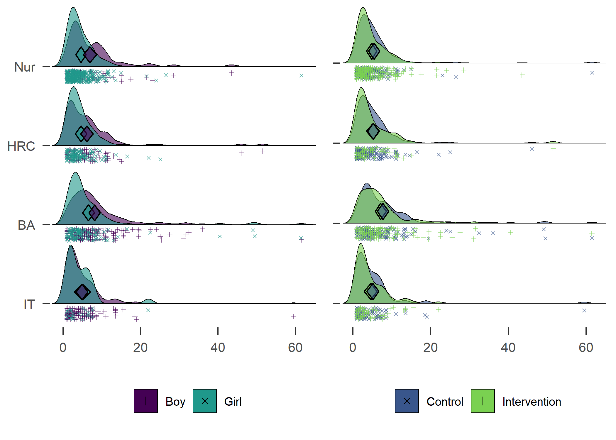
Self-reported minutes of MVPA during the previous week. Nur = Practical nurse, HRC = Hotel, restaurant and catering, BA = Business and administration, IT = Information and communications technology.

Self-reported minutes of MVPA during the previous week. Nur = Practical nurse, HRC = Hotel, restaurant and catering, BA = Business and administration, IT = Information and communications technology.

Breaks in sedentary time

This section reports the accelerometer-measured number of breaks to sitting time.

Data preparation

Description

The tab “Information on data preparation” of this section present information on data preparation for the plot

Information on data preparation

Code chunk below prepares data.

# m_sitBreaksAccelerometer_trackgirl <- brms::bf(sitBreaksAccelerometer_T1 ~ (1 | track:girl)) %>% 
#   brms::brm(., data = df, chains = 4, iter = 4000, control = list(adapt_delta = 0.95))
# 
# brms::prior_summary(m_sitBreaksAccelerometer_trackgirl, data = df)
# 
# m_sitBreaksAccelerometer_trackgirl
# 
# b_intercept <- brms::fixef(m_sitBreaksAccelerometer_trackgirl)[1]
# 
# # This gives estimates only:
# sitBreaksAccelerometer_trackgirl_estimates <- brms::ranef(m_sitBreaksAccelerometer_trackgirl)[[1]][1:10]
# 
# # The 2.5%ile:
# sitBreaksAccelerometer_trackgirl_CIL <- brms::ranef(m_sitBreaksAccelerometer_trackgirl)[[1]][21:30]
# 
# # The 97.5%ile:
# sitBreaksAccelerometer_trackgirl_CIH <- brms::ranef(m_sitBreaksAccelerometer_trackgirl)[[1]][31:40]
# 
# sitBreaksAccelerometer_trackgirl_ci <- data.frame(sitBreaksAccelerometer_trackgirl_CIL, sitBreaksAccelerometer_trackgirl_estimates, sitBreaksAccelerometer_trackgirl_CIH, Variable = labels(brms::ranef(m_sitBreaksAccelerometer_trackgirl))) %>% 
#   dplyr::mutate(b_intercept = rep(b_intercept, 10)) %>% 
#   dplyr::mutate(sitBreaksAccelerometer_trackgirl_CIL = sitBreaksAccelerometer_trackgirl_CIL + b_intercept,
#          sitBreaksAccelerometer_trackgirl_estimates = sitBreaksAccelerometer_trackgirl_estimates + b_intercept,
#          sitBreaksAccelerometer_trackgirl_CIH = sitBreaksAccelerometer_trackgirl_CIH + b_intercept,
#          track = c('BA_boy',
#                    'BA_girl',
#                    'HRC_boy',
#                    'HRC_girl',
#                    'IT_boy',
#                    'IT_girl',
#                    'Nur_boy',
#                    'Nur_girl',
#                    'Other_boy',
#                    'Other_girl'
# ))
# 
# sitBreaksAccelerometer_trackgirl_diamonds_girl <- rbind(
# sitBreaksAccelerometer_trackgirl_ci %>% dplyr::filter(track == "Nur_girl"),
# sitBreaksAccelerometer_trackgirl_ci %>% dplyr::filter(track == "HRC_girl"),
# sitBreaksAccelerometer_trackgirl_ci %>% dplyr::filter(track == "BA_girl"),
# sitBreaksAccelerometer_trackgirl_ci %>% dplyr::filter(track == "IT_girl")) %>% 
#   arrange(-row_number()) # reverse order of rows to make them right for the plot to come
# 
# sitBreaksAccelerometer_trackgirl_diamonds_boy <- rbind(
# sitBreaksAccelerometer_trackgirl_ci %>% dplyr::filter(track == "Nur_boy"),
# sitBreaksAccelerometer_trackgirl_ci %>% dplyr::filter(track == "HRC_boy"),
# sitBreaksAccelerometer_trackgirl_ci %>% dplyr::filter(track == "BA_boy"),
# sitBreaksAccelerometer_trackgirl_ci %>% dplyr::filter(track == "IT_boy")) %>% 
#   arrange(-row_number()) # reverse order of rows to make them right for the plot to come
# 
# 
# m_sitBreaksAccelerometer_trackintervention <- brms::bf(sitBreaksAccelerometer_T1 ~ (1 | track:intervention)) %>% 
#   brms::brm(., data = df, chains = 4, iter = 4000, control = list(adapt_delta = 0.95))
# 
# brms::prior_summary(m_sitBreaksAccelerometer_trackintervention, data = df)
# 
# m_sitBreaksAccelerometer_trackintervention
# 
# b_intercept <- brms::fixef(m_sitBreaksAccelerometer_trackintervention)[1]
# 
# # This gives estimates only:
# sitBreaksAccelerometer_trackintervention_estimates <- brms::ranef(m_sitBreaksAccelerometer_trackintervention)[[1]][1:10]
# 
# # The 2.5%ile:
# sitBreaksAccelerometer_trackintervention_CIL <- brms::ranef(m_sitBreaksAccelerometer_trackintervention)[[1]][21:30]
# 
# # The 97.5%ile:
# sitBreaksAccelerometer_trackintervention_CIH <- brms::ranef(m_sitBreaksAccelerometer_trackintervention)[[1]][31:40]
# 
# sitBreaksAccelerometer_trackintervention_ci <- data.frame(sitBreaksAccelerometer_trackintervention_CIL, sitBreaksAccelerometer_trackintervention_estimates, sitBreaksAccelerometer_trackintervention_CIH, Variable = labels(brms::ranef(m_sitBreaksAccelerometer_trackintervention))) %>% 
#   dplyr::mutate(b_intercept = rep(b_intercept, 10)) %>% 
#   dplyr::mutate(sitBreaksAccelerometer_trackintervention_CIL = sitBreaksAccelerometer_trackintervention_CIL + b_intercept,
#          sitBreaksAccelerometer_trackintervention_estimates = sitBreaksAccelerometer_trackintervention_estimates + b_intercept,
#          sitBreaksAccelerometer_trackintervention_CIH = sitBreaksAccelerometer_trackintervention_CIH + b_intercept,
#          track = c('BA_control',
#                    'BA_intervention',
#                    'HRC_control',
#                    'HRC_intervention',
#                    'IT_control',
#                    'IT_intervention',
#                    'Nur_control',
#                    'Nur_intervention',
#                    'Other_control',
#                    'Other_intervention'
# ))
# 
# sitBreaksAccelerometer_trackintervention_diamonds_intervention <- rbind(
# sitBreaksAccelerometer_trackintervention_ci %>% dplyr::filter(track == "Nur_intervention"),
# sitBreaksAccelerometer_trackintervention_ci %>% dplyr::filter(track == "HRC_intervention"),
# sitBreaksAccelerometer_trackintervention_ci %>% dplyr::filter(track == "BA_intervention"),
# sitBreaksAccelerometer_trackintervention_ci %>% dplyr::filter(track == "IT_intervention")) %>% 
#   arrange(-row_number()) # reverse order of rows to make them right for the plot to come
# 
# sitBreaksAccelerometer_trackintervention_diamonds_control <- rbind(
# sitBreaksAccelerometer_trackintervention_ci %>% dplyr::filter(track == "Nur_control"),
# sitBreaksAccelerometer_trackintervention_ci %>% dplyr::filter(track == "HRC_control"),
# sitBreaksAccelerometer_trackintervention_ci %>% dplyr::filter(track == "BA_control"),
# sitBreaksAccelerometer_trackintervention_ci %>% dplyr::filter(track == "IT_control")) %>% 
#   arrange(-row_number()) # reverse order of rows to make them right for the plot to come
# 
# save(sitBreaksAccelerometer_trackgirl_diamonds_girl, file = "./Rdata_files/sitBreaksAccelerometer_trackgirl_diamonds_girl.Rdata")
# save(sitBreaksAccelerometer_trackgirl_diamonds_boy, file = "./Rdata_files/sitBreaksAccelerometer_trackgirl_diamonds_boy.Rdata")
# save(sitBreaksAccelerometer_trackintervention_diamonds_intervention, file = "./Rdata_files/sitBreaksAccelerometer_trackintervention_diamonds_intervention.Rdata")
# save(sitBreaksAccelerometer_trackintervention_diamonds_control, file = "./Rdata_files/sitBreaksAccelerometer_trackintervention_diamonds_control.Rdata")

load("./Rdata_files/sitBreaksAccelerometer_trackgirl_diamonds_girl.Rdata")
load("./Rdata_files/sitBreaksAccelerometer_trackgirl_diamonds_boy.Rdata")
load("./Rdata_files/sitBreaksAccelerometer_trackintervention_diamonds_intervention.Rdata")
load("./Rdata_files/sitBreaksAccelerometer_trackintervention_diamonds_control.Rdata")

Density plot by intervention and gender


# Create data frame
densplot <- d
levels(densplot$intervention) <- c("Control", "Intervention")
levels(densplot$girl) <- recode(densplot$girl, "boy" = "Boys", "girl" = "Girls")

# This gives side-by-side plots. There's a third plot below the two, which is fake to include x-axis text.
layout(matrix(c(1, 2, 3, 3), nrow = 2, ncol = 2, byrow = TRUE),
       widths = c(0.5, 0.5), heights = c(0.45, 0.05))

# Minimise whitespace; see https://stackoverflow.com/questions/15848942/how-to-reduce-space-gap-between-multiple-graphs-in-r
par(mai = c(0.3, 0.3, 0.1, 0.0)) 

## Girls vs. boys
# Choose only the variables needed and drop NA
dens <- densplot %>% dplyr::select(sitBreaksAccelerometer_T1, girl) %>% 
  dplyr::filter(complete.cases(.))

# Set random number generator for reproducibility of bootstrap test of equal densities
set.seed(10)

# Make plot
sm.sitBreaksAccelerometer_T1_2 <- sm.density.compare2(as.numeric(dens$sitBreaksAccelerometer_T1), 
                                               as.factor(dens$girl), 
                                               model = "equal",
                                               xlab = "", ylab = "",
                                               col = viridis::viridis(4, end  =  0.8)[c(3, 1)], 
                                               lty = c(1, 3), yaxt = "n",
                                               bandcol = 'LightGray', 
                                               lwd = c(2, 2))
## 
## Test of equal densities:  p-value =  0
legend("topright", levels(dens$girl), col = viridis::viridis(4, end = 0.8)[c(1, 3)], lty = c(3,1), lwd = (c(2,2)))
mtext(side = 2, "Density", line = 0.5)

## Intervention vs. control
# Choose only the variables needed and drop NA
dens <- densplot %>% dplyr::select(sitBreaksAccelerometer_T1, intervention) %>% 
  dplyr::filter(complete.cases(.))

# Set random number generator for reproducibility of bootstrap test of equal densities
set.seed(10)
# Make plot
sm.sitBreaksAccelerometer_T1_2 <- sm.density.compare2(as.numeric(dens$sitBreaksAccelerometer_T1), 
                                               as.factor(dens$intervention), 
                                               model = "equal", 
                                               xlab = "", ylab = "",
                                               col = viridis::viridis(4, end = 0.8)[c(2, 4)], 
                                               lty = c(3, 1), yaxt = "n",
                                               bandcol = 'LightGray', 
                                               lwd = c(2, 2))
## 
## Test of equal densities:  p-value =  0.01
legend("topright", levels(dens$intervention), col = viridis::viridis(4, end = 0.8)[c(2, 4)], lty=c(3,1), lwd=(c(2,2)))

# Create x-axis label. See https://stackoverflow.com/questions/11198767/how-to-annotate-across-or-between-plots-in-multi-plot-panels-in-r
par(mar = c(0,0,0,0)) 
plot(1, 1, type = "n", frame.plot = FALSE, axes = FALSE) # Fake plot for x-axis label
text(x = 1.02, y = 1.3, labels = "Average number of breaks in daily sitting", pos = 1)
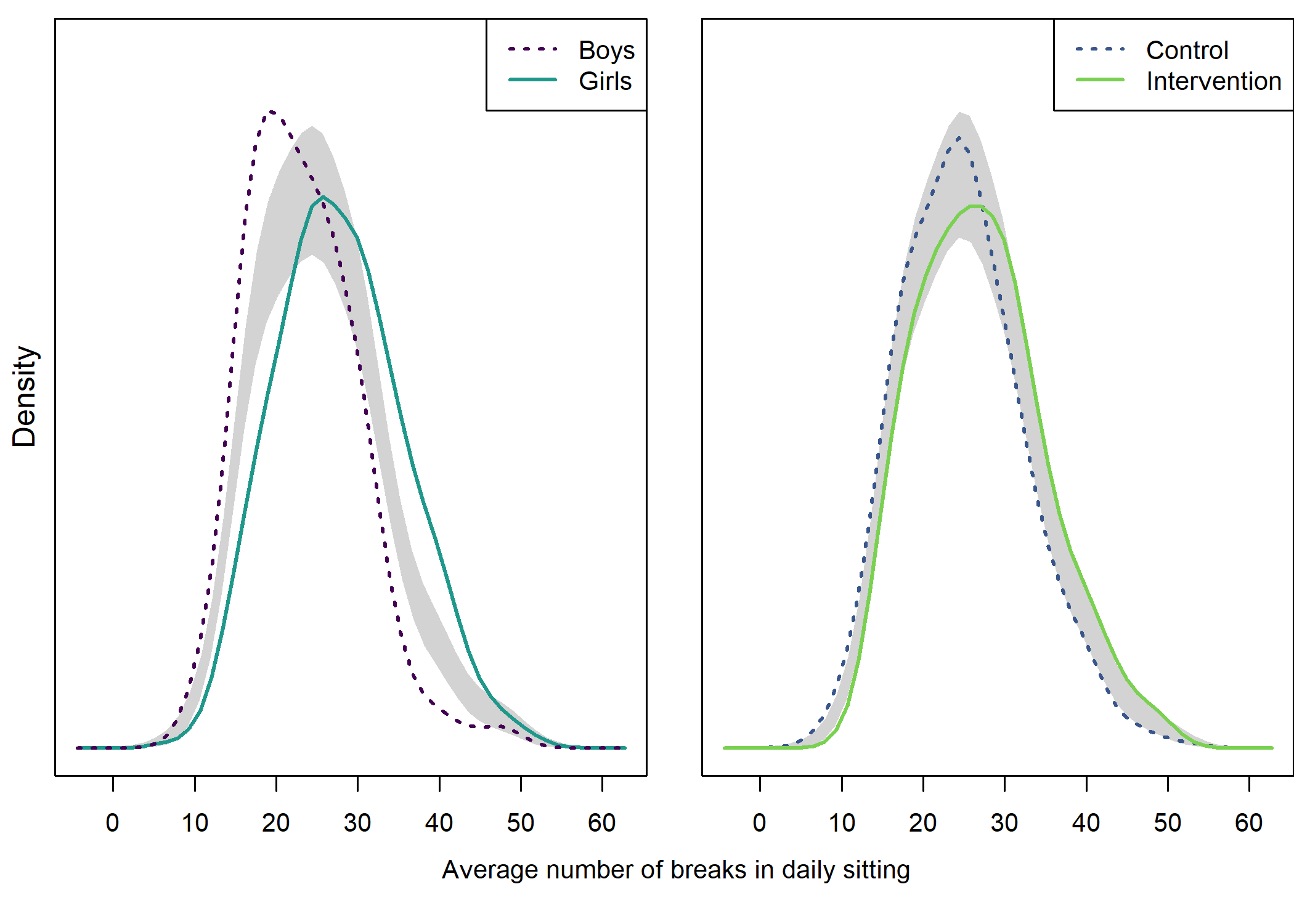
Density plot by track


plot1 <- df %>% dplyr::select(id,
                              track = track,
                              girl,
                              PA = sitBreaksAccelerometer_T1)  %>%
  dplyr::filter(!is.na(track), track != "Other") %>% # Drop category "Other"
  dplyr::mutate(track = factor(track, levels = c("IT", "BA", "HRC", "Nur")),
                track = recode_factor(track, "IT" = "IT", "BA" = "BA", 
                                      "HRC" = "HRC", "Nur" = "Nur")) %>% 
  ggplot2::ggplot(aes(y = track)) +
  ggridges::geom_density_ridges2(aes(x = PA, colour = "black", 
                                    fill = paste(track, girl),
                                    point_color = girl,
                                    point_fill = girl,
                                    point_shape = girl),
                                  scale = .6, alpha = 0.6, size = 0.25,
                                  position = position_raincloud(width = 0.2, height = 0.15),
                                  # from = 0, to = 450,
                                  jittered_points = TRUE,
                                  point_size = 1) +
  labs(x = NULL,
       y = NULL) +
  scale_y_discrete(expand = c(0.1, 0)) +
  scale_x_continuous(expand = c(0.01, 0)) +
  ggridges::scale_fill_cyclical(
                                labels = c('BA boy' = "Boy", 'BA girl' = "Girl"),
                                values = viridis::viridis(4, end = 0.8)[c(1, 3)],
                                name = "", 
                                guide = guide_legend(override.aes = list(alpha = 1, 
                                                                         point_shape = c(3, 4),
                                                                         point_size = 2))) +
  ggridges::scale_colour_cyclical(values = "black") +
  ggridges::theme_ridges(grid = FALSE) +
  # ggplot2::scale_fill_manual(values = c("#A0FFA0", "#A0A0FF")) +
  ggridges::scale_discrete_manual(aesthetics = "point_color", 
                                  values = viridis::viridis(4, end = 0.8)[c(3, 1)],
                                  guide = "none") +
  ggridges::scale_discrete_manual(aesthetics = "point_fill",
                                  values = viridis::viridis(4, end = 0.8)[c(3, 1)],
                                  guide = "none") +
  ggridges::scale_discrete_manual(aesthetics = "point_shape", 
                                  values = c(4, 3),
                                  guide = "none") +
  papaja::theme_apa() +
  theme(legend.position = "bottom")

plot1 <- plot1 + 
  userfriendlyscience::diamondPlot(sitBreaksAccelerometer_trackgirl_diamonds_girl, 
                                   returnLayerOnly = TRUE, 
                                   lineColor = "black", 
                                   color=viridis::viridis(4, end = 0.8)[3],
                                   alpha=.6, 
                                   fixedSize = 0.1, 
                                   otherAxisCol = (1:4 + .15)) + # specify y-position; option to move the diamond 
  userfriendlyscience::diamondPlot(sitBreaksAccelerometer_trackgirl_diamonds_boy, 
                                   returnLayerOnly = TRUE, 
                                   lineColor = "black", 
                                   linetype = "solid", 
                                   color=viridis::viridis(4, end = 0.8)[1],
                                   alpha=.6, 
                                   fixedSize = 0.1, 
                                   otherAxisCol = (1:4 + .15))

# Draw plot with intervention and control densities

plot2 <- df %>% dplyr::select(id,
                              track = track,
                              intervention,
                              PA = sitBreaksAccelerometer_T1)  %>%
  dplyr::filter(!is.na(track), track != "Other") %>% # Drop category "Other"
  dplyr::mutate(track = factor(track, levels = c("IT", "BA", "HRC", "Nur")),
                track = recode_factor(track, "IT" = "IT", "BA" = "BA", 
                                      "HRC" = "HRC", "Nur" = "Nur")) %>% 
  ggplot2::ggplot(aes(y = track)) +
  ggridges::geom_density_ridges2(aes(x = PA, colour = "black", 
                                    fill = paste(track, intervention),
                                    point_color = intervention,
                                    point_fill = intervention,
                                    point_shape = intervention),
                                  scale = .6, alpha = 0.6, size = 0.25,
                                  position = position_raincloud(width = 0.2, height = 0.15),
                                  # from = 0, to = 450,
                                  jittered_points = TRUE,
                                  point_size = 1) +
  labs(x = NULL,
       y = NULL) +
  scale_y_discrete(expand = c(0.1, 0), labels = NULL) +
  scale_x_continuous(expand = c(0.01, 0)) +
  ggridges::scale_fill_cyclical(
                                labels = c('BA 0' = "Control", 'BA 1' = "Intervention"),
                                values = viridis::viridis(4, end = 0.8)[c(2, 4)],
                                name = "", 
                                guide = guide_legend(override.aes = list(alpha = 1, 
                                                                         point_shape = c(4, 3),
                                                                         point_size = 2))) +
  ggridges::scale_colour_cyclical(values = "black") +
  ggridges::theme_ridges(grid = FALSE) +
  # ggplot2::scale_fill_manual(values = c("#A0FFA0", "#A0A0FF")) +
  ggridges::scale_discrete_manual(aesthetics = "point_color", 
                                  values = viridis::viridis(4, end = 0.8)[c(2, 4)],
                                  guide = "none") +
  ggridges::scale_discrete_manual(aesthetics = "point_fill",
                                  values = viridis::viridis(4, end = 0.8)[c(2, 4)],
                                  guide = "none") +
  ggridges::scale_discrete_manual(aesthetics = "point_shape", 
                                  values = c(4, 3),
                                  guide = "none") +
  papaja::theme_apa() +
  theme(legend.position = "bottom")

plot2 <- plot2 + 
  userfriendlyscience::diamondPlot(sitBreaksAccelerometer_trackintervention_diamonds_intervention, 
                                   returnLayerOnly = TRUE, 
                                   lineColor = "black",  
                                   color=viridis::viridis(4, end = 0.8)[4],
                                   alpha=.6, 
                                   fixedSize = 0.1, 
                                   otherAxisCol = (1:4 + .15)) +
  userfriendlyscience::diamondPlot(sitBreaksAccelerometer_trackintervention_diamonds_control, 
                                   returnLayerOnly = TRUE, 
                                   lineColor = "black",  
                                   color=viridis::viridis(4, end = 0.8)[2],
                                   alpha=.6, 
                                   fixedSize = 0.1, 
                                   otherAxisCol = (1:4 + .15))

plot1 + plot2
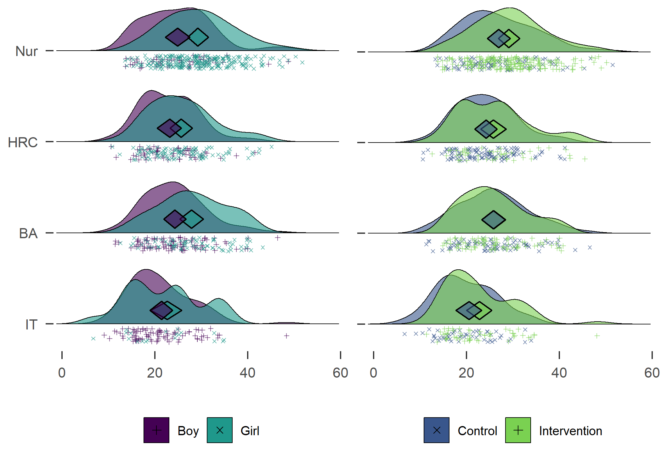
Breaks in sedentary time. Nur = Practical nurse, HRC = Hotel, restaurant and catering, BA = Business and administration, IT = Information and communications technology.

Breaks in sedentary time. Nur = Practical nurse, HRC = Hotel, restaurant and catering, BA = Business and administration, IT = Information and communications technology.

Girls in all educational tracks interrupted sitting more than boys.

SB, Accelerometer-measured

Density plot by intervention and gender


# Create data frame
densplot <- d
levels(densplot$intervention) <- c("Control", "Intervention")
levels(densplot$girl) <- recode(densplot$girl, "boy" = "Boys", "girl" = "Girls")

# This gives side-by-side plots. There's a third plot below the two, which is fake to include x-axis text.
layout(matrix(c(1, 2, 3, 3), nrow = 2, ncol = 2, byrow = TRUE),
       widths = c(0.5, 0.5), heights = c(0.45, 0.05))

# Minimise whitespace; see https://stackoverflow.com/questions/15848942/how-to-reduce-space-gap-between-multiple-graphs-in-r
par(mai = c(0.3, 0.3, 0.1, 0.0)) 

## Girls vs. boys
# Choose only the variables needed and drop NA
dens <- densplot %>% dplyr::select(sitLieAccelerometer_T1, girl) %>% 
  dplyr::filter(complete.cases(.))

# Set random number generator for reproducibility of bootstrap test of equal densities
set.seed(10)

# Make plot
sm.sitLieAccelerometer_T1_2 <- sm.density.compare2(as.numeric(dens$sitLieAccelerometer_T1), 
                                               as.factor(dens$girl), 
                                               model = "equal",
                                               xlab = "", ylab = "",
                                               col = viridis::viridis(4, end  =  0.8)[c(3, 1)], 
                                               lty = c(1, 3), yaxt = "n",
                                               bandcol = 'LightGray', 
                                               lwd = c(2, 2))
## 
## Test of equal densities:  p-value =  0
legend("topright", levels(dens$girl), col = viridis::viridis(4, end = 0.8)[c(1, 3)], lty = c(3,1), lwd = (c(2,2)))
mtext(side = 2, "Density", line = 0.5)

## Intervention vs. control
# Choose only the variables needed and drop NA
dens <- densplot %>% dplyr::select(sitLieAccelerometer_T1, intervention) %>% 
  dplyr::filter(complete.cases(.))

# Set random number generator for reproducibility of bootstrap test of equal densities
set.seed(10)
# Make plot
sm.sitLieAccelerometer_T1_2 <- sm.density.compare2(as.numeric(dens$sitLieAccelerometer_T1), 
                                               as.factor(dens$intervention), 
                                               model = "equal", 
                                               xlab = "", ylab = "",
                                               col = viridis::viridis(4, end = 0.8)[c(2, 4)], 
                                               lty = c(3, 1), yaxt = "n",
                                               bandcol = 'LightGray', 
                                               lwd = c(2, 2))
## 
## Test of equal densities:  p-value =  0.07
legend("topright", levels(dens$intervention), col = viridis::viridis(4, end = 0.8)[c(2, 4)], lty=c(3,1), lwd=(c(2,2)))

# Create x-axis label. See https://stackoverflow.com/questions/11198767/how-to-annotate-across-or-between-plots-in-multi-plot-panels-in-r
par(mar = c(0,0,0,0)) 
plot(1, 1, type = "n", frame.plot = FALSE, axes = FALSE) # Fake plot for x-axis label
text(x = 1.02, y = 1.3, labels = "Average daily hours spent sitting or lying down", pos = 1)
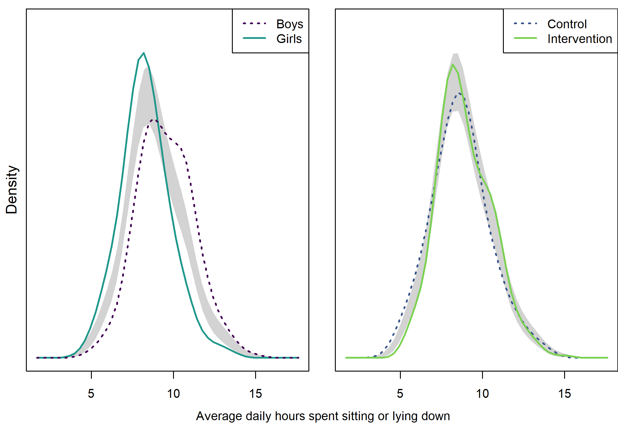
Differences in time spent sitting and lying down emerged between boys and girls, the former spending more time being sedentary. Even though there was some heterogeneity among schools, again the aggregated intervention and control schools showed no differences.

Data preparation

Description

The tab “Information on data preparation” of this section present information on data preparation for the plot

Information on data preparation

Prepare data: time spent sitting & lying down

Get credibility intervals track:school

# m_sitLieAccelerometer_trackgirl <- brms::bf(sitLieAccelerometer_T1 ~ (1 | track:girl)) %>% 
#   brms::brm(., data = df, chains = 4, iter = 4000, control = list(adapt_delta = 0.95))
# 
# brms::prior_summary(m_sitLieAccelerometer_trackgirl, data = df)
# 
# m_sitLieAccelerometer_trackgirl
# 
# b_intercept <- brms::fixef(m_sitLieAccelerometer_trackgirl)[1]
# 
# # This gives estimates only:
# sitLie_trackgirl_estimates <- brms::ranef(m_sitLieAccelerometer_trackgirl)[[1]][1:10]
# 
# # The 2.5%ile:
# sitLie_trackgirl_CIL <- brms::ranef(m_sitLieAccelerometer_trackgirl)[[1]][21:30]
# 
# # The 97.5%ile:
# sitLie_trackgirl_CIH <- brms::ranef(m_sitLieAccelerometer_trackgirl)[[1]][31:40]
# 
# sitLie_trackgirl_ci <- data.frame(sitLie_trackgirl_CIL, sitLie_trackgirl_estimates, sitLie_trackgirl_CIH, Variable = labels(brms::ranef(m_sitLieAccelerometer_trackgirl))) %>% 
#   dplyr::mutate(b_intercept = rep(b_intercept, 10)) %>% 
#   dplyr::mutate(sitLie_trackgirl_CIL = sitLie_trackgirl_CIL + b_intercept,
#          sitLie_trackgirl_estimates = sitLie_trackgirl_estimates + b_intercept,
#          sitLie_trackgirl_CIH = sitLie_trackgirl_CIH + b_intercept,
#          track = c('BA_boy',
#                    'BA_girl',
#                    'HRC_boy',
#                    'HRC_girl',
#                    'IT_boy',
#                    'IT_girl',
#                    'Nur_boy',
#                    'Nur_girl',
#                    'Other_boy',
#                    'Other_girl'
# ))
# 
# sitLie_trackgirl_diamonds_girl <- rbind(
# sitLie_trackgirl_ci %>% dplyr::filter(track == "Nur_girl"),
# sitLie_trackgirl_ci %>% dplyr::filter(track == "HRC_girl"),
# sitLie_trackgirl_ci %>% dplyr::filter(track == "BA_girl"),
# sitLie_trackgirl_ci %>% dplyr::filter(track == "IT_girl")) %>% 
#   arrange(-row_number()) # reverse order of rows to make them right for the plot to come
# 
# sitLie_trackgirl_diamonds_boy <- rbind(
# sitLie_trackgirl_ci %>% dplyr::filter(track == "Nur_boy"),
# sitLie_trackgirl_ci %>% dplyr::filter(track == "HRC_boy"),
# sitLie_trackgirl_ci %>% dplyr::filter(track == "BA_boy"),
# sitLie_trackgirl_ci %>% dplyr::filter(track == "IT_boy")) %>% 
#   arrange(-row_number()) # reverse order of rows to make them right for the plot to come
# 
# 
# m_sitLieAccelerometer_trackintervention <- brms::bf(sitLieAccelerometer_T1 ~ (1 | track:intervention)) %>% 
#   brms::brm(., data = df, chains = 4, iter = 4000, control = list(adapt_delta = 0.95))
# 
# brms::prior_summary(m_sitLieAccelerometer_trackintervention, data = df)
# 
# m_sitLieAccelerometer_trackintervention
# 
# b_intercept <- brms::fixef(m_sitLieAccelerometer_trackintervention)[1]
# 
# # This gives estimates only:
# sitLie_trackintervention_estimates <- brms::ranef(m_sitLieAccelerometer_trackintervention)[[1]][1:10]
# 
# 
# # The 2.5%ile:
# sitLie_trackintervention_CIL <- brms::ranef(m_sitLieAccelerometer_trackintervention)[[1]][21:30]
# 
# # The 97.5%ile:
# sitLie_trackintervention_CIH <- brms::ranef(m_sitLieAccelerometer_trackintervention)[[1]][31:40]
# 
# sitLie_trackintervention_ci <- data.frame(sitLie_trackintervention_CIL, sitLie_trackintervention_estimates, sitLie_trackintervention_CIH, Variable = labels(brms::ranef(m_sitLieAccelerometer_trackintervention))) %>% 
#   dplyr::mutate(b_intercept = rep(b_intercept, 10)) %>% 
#   dplyr::mutate(sitLie_trackintervention_CIL = sitLie_trackintervention_CIL + b_intercept,
#          sitLie_trackintervention_estimates = sitLie_trackintervention_estimates + b_intercept,
#          sitLie_trackintervention_CIH = sitLie_trackintervention_CIH + b_intercept,
#          track = c('BA_control',
#                    'BA_intervention',
#                    'HRC_control',
#                    'HRC_intervention',
#                    'IT_control',
#                    'IT_intervention',
#                    'Nur_control',
#                    'Nur_intervention',
#                    'Other_control',
#                    'Other_intervention'
# ))
# 
# sitLie_trackintervention_diamonds_intervention <- rbind(
# sitLie_trackintervention_ci %>% dplyr::filter(track == "Nur_intervention"),
# sitLie_trackintervention_ci %>% dplyr::filter(track == "HRC_intervention"),
# sitLie_trackintervention_ci %>% dplyr::filter(track == "BA_intervention"),
# sitLie_trackintervention_ci %>% dplyr::filter(track == "IT_intervention")) %>% 
#   arrange(-row_number()) # reverse order of rows to make them right for the plot to come
# 
# sitLie_trackintervention_diamonds_control <- rbind(
# sitLie_trackintervention_ci %>% dplyr::filter(track == "Nur_control"),
# sitLie_trackintervention_ci %>% dplyr::filter(track == "HRC_control"),
# sitLie_trackintervention_ci %>% dplyr::filter(track == "BA_control"),
# sitLie_trackintervention_ci %>% dplyr::filter(track == "IT_control")) %>% 
#   arrange(-row_number()) # reverse order of rows to make them right for the plot to come
# 
# save(sitLie_trackgirl_diamonds_girl, file = "./Rdata_files/sitLie_trackgirl_diamonds_girl.Rdata")
# save(sitLie_trackgirl_diamonds_boy, file = "./Rdata_files/sitLie_trackgirl_diamonds_boy.Rdata")
# save(sitLie_trackintervention_diamonds_intervention, file = "./Rdata_files/sitLie_trackintervention_diamonds_intervention.Rdata")
# save(sitLie_trackintervention_diamonds_control, file = "./Rdata_files/sitLie_trackintervention_diamonds_control.Rdata")

load("./Rdata_files/sitLie_trackgirl_diamonds_girl.Rdata")
load("./Rdata_files/sitLie_trackgirl_diamonds_boy.Rdata")
load("./Rdata_files/sitLie_trackintervention_diamonds_intervention.Rdata")
load("./Rdata_files/sitLie_trackintervention_diamonds_control.Rdata")

Basic observed characteristics

NOTE: These values do not account for clustering.

Density plot by track

Time spent sitting or lying down


plot1 <- df %>% dplyr::select(id,
                              track = track,
                              girl,
                              PA = sitLieAccelerometer_T1)  %>%
  dplyr::filter(!is.na(track), track != "Other") %>% # Drop category "Other"
  dplyr::mutate(track = factor(track, levels = c("IT", "BA", "HRC", "Nur")),
                track = recode_factor(track, "IT" = "IT", "BA" = "BA", 
                                      "HRC" = "HRC", "Nur" = "Nur")) %>% 
  ggplot2::ggplot(aes(y = track)) +
  ggridges::geom_density_ridges2(aes(x = PA, colour = "black", 
                                    fill = paste(track, girl),
                                    point_color = girl,
                                    point_fill = girl,
                                    point_shape = girl),
                                  scale = .75, alpha = 0.6, size = 0.25,
                                  position = position_raincloud(width = 0.05, height = 0.15),
                                  # from = 0, to = 450,
                                  jittered_points = TRUE,
                                  point_size = 1) +
  labs(x = NULL,
       y = NULL) +
  scale_y_discrete(expand = c(0.1, 0)) +
  scale_x_continuous(expand = c(0.01, 0)) +
  ggridges::scale_fill_cyclical(
                                labels = c('BA boy' = "Boy", 'BA girl' = "Girl"),
                                values = viridis::viridis(4, end = 0.8)[c(1, 3)],
                                name = "", 
                                guide = guide_legend(override.aes = list(alpha = 1, 
                                                                         point_shape = c(3, 4),
                                                                         point_size = 2))) +
  ggridges::scale_colour_cyclical(values = "black") +
  ggridges::theme_ridges(grid = FALSE) +
  # ggplot2::scale_fill_manual(values = c("#A0FFA0", "#A0A0FF")) +
  ggridges::scale_discrete_manual(aesthetics = "point_color", 
                                  values = viridis::viridis(4, end = 0.8)[c(3, 1)],
                                  guide = "none") +
  ggridges::scale_discrete_manual(aesthetics = "point_fill",
                                  values = viridis::viridis(4, end = 0.8)[c(3, 1)],
                                  guide = "none") +
  ggridges::scale_discrete_manual(aesthetics = "point_shape", 
                                  values = c(4, 3),
                                  guide = "none") +
  papaja::theme_apa() +
  theme(legend.position = "bottom")

sitLie_trackgirl_diamonds_girl_hours <- sitLie_trackgirl_diamonds_girl %>% 
  dplyr::mutate_if(is.numeric, ~./60)
sitLie_trackgirl_diamonds_boy_hours <- sitLie_trackgirl_diamonds_boy %>% 
  dplyr::mutate_if(is.numeric, ~./60)

plot1 <- plot1 + 
  userfriendlyscience::diamondPlot(sitLie_trackgirl_diamonds_girl_hours, 
                                   returnLayerOnly = TRUE, 
                                   lineColor = "black", 
                                   color=viridis::viridis(4, end = 0.8)[3],
                                   alpha=.6, 
                                   fixedSize = 0.1, 
                                   otherAxisCol = (1:4 + .15)) + # specify y-position; option to move the diamond 
  userfriendlyscience::diamondPlot(sitLie_trackgirl_diamonds_boy_hours, 
                                   returnLayerOnly = TRUE, 
                                   lineColor = "black", 
                                   linetype = "solid", 
                                   color=viridis::viridis(4, end = 0.8)[1],
                                   alpha=.6, 
                                   fixedSize = 0.1, 
                                   otherAxisCol = (1:4 + .15))

# Draw plot with intervention and control densities

plot2 <- df %>% dplyr::select(id,
                              track = track,
                              intervention,
                              PA = sitLieAccelerometer_T1)  %>%
  dplyr::filter(!is.na(track), track != "Other") %>% # Drop category "Other"
  dplyr::mutate(track = factor(track, levels = c("IT", "BA", "HRC", "Nur")),
                track = recode_factor(track, "IT" = "IT", "BA" = "BA", 
                                      "HRC" = "HRC", "Nur" = "Nur")) %>% 
  ggplot2::ggplot(aes(y = track)) +
  ggridges::geom_density_ridges2(aes(x = PA, colour = "black", 
                                    fill = paste(track, intervention),
                                    point_color = intervention,
                                    point_fill = intervention,
                                    point_shape = intervention),
                                  scale = .75, alpha = 0.6, size = 0.25,
                                  position = position_raincloud(width = 0.05, height = 0.15),
                                  # from = 0, to = 450,
                                  jittered_points = TRUE,
                                  point_size = 1) +
  labs(x = NULL,
       y = NULL) +
  scale_y_discrete(expand = c(0.1, 0), labels = NULL) +
  scale_x_continuous(expand = c(0.01, 0)) +
  ggridges::scale_fill_cyclical(
                                labels = c('BA 0' = "Control", 'BA 1' = "Intervention"),
                                values = viridis::viridis(4, end = 0.8)[c(2, 4)],
                                name = "", 
                                guide = guide_legend(override.aes = list(alpha = 1, 
                                                                         point_shape = c(4, 3),
                                                                         point_size = 2))) +
  ggridges::scale_colour_cyclical(values = "black") +
  ggridges::theme_ridges(grid = FALSE) +
  # ggplot2::scale_fill_manual(values = c("#A0FFA0", "#A0A0FF")) +
  ggridges::scale_discrete_manual(aesthetics = "point_color", 
                                  values = viridis::viridis(4, end = 0.8)[c(2, 4)],
                                  guide = "none") +
  ggridges::scale_discrete_manual(aesthetics = "point_fill",
                                  values = viridis::viridis(4, end = 0.8)[c(2, 4)],
                                  guide = "none") +
  ggridges::scale_discrete_manual(aesthetics = "point_shape", 
                                  values = c(4, 3),
                                  guide = "none") +
  papaja::theme_apa() +
  theme(legend.position = "bottom")

sitLie_trackintervention_diamonds_intervention_hours <- sitLie_trackintervention_diamonds_intervention %>% 
  dplyr::mutate_if(is.numeric, ~./60)
sitLie_trackintervention_diamonds_control_hours <- sitLie_trackintervention_diamonds_control %>% 
  dplyr::mutate_if(is.numeric, ~./60)

plot2 <- plot2 + 
  userfriendlyscience::diamondPlot(sitLie_trackintervention_diamonds_intervention, 
                                   returnLayerOnly = TRUE, 
                                   lineColor = "black",  
                                   color=viridis::viridis(4, end = 0.8)[4],
                                   alpha=.6, 
                                   fixedSize = 0.1, 
                                   otherAxisCol = (1:4 + .15)) +
  userfriendlyscience::diamondPlot(sitLie_trackintervention_diamonds_control, 
                                   returnLayerOnly = TRUE, 
                                   lineColor = "black",  
                                   color=viridis::viridis(4, end = 0.8)[2],
                                   alpha=.6, 
                                   fixedSize = 0.1, 
                                   otherAxisCol = (1:4 + .15))

plot1 + plot2
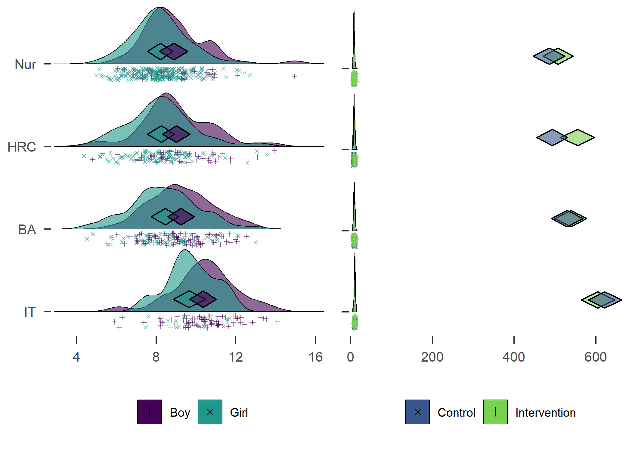
Average time spent sitting or lying down during a day. Nur = Practical nurse, HRC = Hotel, restaurant and catering, BA = Business and administration, IT = Information and communications technology.

Average time spent sitting or lying down during a day. Nur = Practical nurse, HRC = Hotel, restaurant and catering, BA = Business and administration, IT = Information and communications technology.

Breaking the distributions down by tracks, this is what we see: boys are more sedentary in all groups, but the IT group–which consists of mostly boys–is also most sedentary regardless of gender. Distributions between intervention and control groups exhibit some differences, but the most pronounced one can be seen in the HRC track.
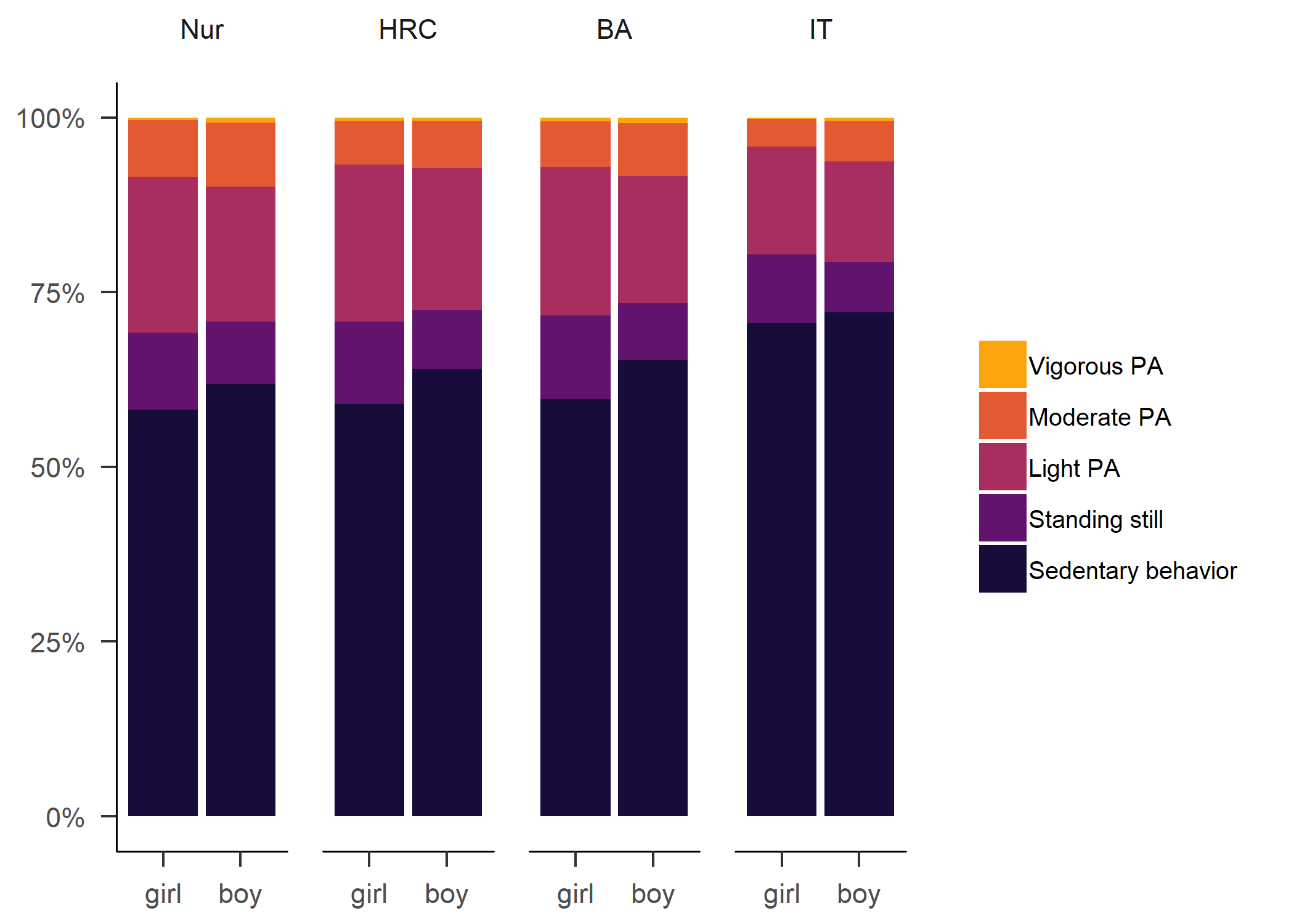
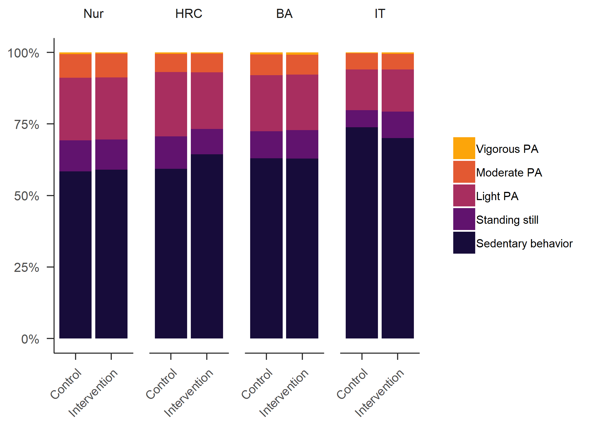
PA Determinants and BCT use

This section reports various hypothesised determinants of physical activity.

Code chunk below loads data written in the section named Tables and Estimators.

Simple diamond plot

Diamonds depict 95% confidence intervals for means.

PA_ci_girls <- ci_girls %>% dplyr::filter(diamondlabels %in% names(scales_T1) & grepl("PA_", diamondlabels) & !grepl("bct", diamondlabels))

PA_ci_boys <- ci_boys %>% dplyr::filter(diamondlabels %in% names(scales_T1) & grepl("PA_", diamondlabels) & !grepl("bct", diamondlabels))

PA_ci_intervention <- ci_intervention %>% dplyr::filter(diamondlabels %in% names(scales_T1) & grepl("PA_", diamondlabels) & !grepl("bct", diamondlabels))

PA_ci_control <- ci_control %>% dplyr::filter(diamondlabels %in% names(scales_T1) & grepl("PA_", diamondlabels) & !grepl("bct", diamondlabels))

ICClabels <- vardatatable_containing_edutrack %>% dplyr::filter(Variable %in% PA_ci_control$diamondlabels)

plot1 <- userfriendlyscience::diamondPlot(PA_ci_girls, color = viridis::viridis(4, end  =  0.8)[3], alpha=.3, yLabels = PA_ci_girls$diamondlabels, fixedSize = 0.3, xlab = NULL) +
  userfriendlyscience::diamondPlot(PA_ci_boys, returnLayerOnly = TRUE, color=viridis::viridis(4, end  =  0.8)[1], alpha=.3, fixedSize = 0.3) +
  scale_x_continuous(limits = c(1, 7), breaks = 1:7)

plot2 <- userfriendlyscience::diamondPlot(PA_ci_intervention, color = viridis::viridis(4, end  =  0.8)[4], alpha=.3, yLabels = c(rep("", length(PA_ci_girls$diamondlabels))), fixedSize = 0.3, xlab = NULL, ylab = NULL) +
  userfriendlyscience::diamondPlot(PA_ci_control, returnLayerOnly = TRUE, color = viridis::viridis(4, end  =  0.8)[2], alpha=.3, fixedSize = 0.3) +
  scale_x_continuous(limits = c(1, 7), breaks = 1:7)

grid::grid.newpage()
grid::grid.draw(cbind(ggplot2::ggplotGrob(plot1), ggplot2::ggplotGrob(plot2), size = "first"))

Boys vs. girls

Diamonds depict 99% confidence intervals for means.

Note: action and coping planning on a scale from 1 to 4.

load("./Rdata_files/ci_total.Rdata")

ci_total_diamond <- ci_total

item_names <- ci_total_diamond %>%
  dplyr::filter(grepl('PA_actionplan_T1|PA_copingplan_T1|PA_agreementDependentBCT_T1|PA_frequencyDependentBCT_T1|PA_amotivation_T1|PA_autonomous_T1|PA_controlled_T1|PA_goal_T1|PA_injunctiveNorm_T1|PA_descriptiveNorm_T1|PA_intention_T1|PA_outcomeExpectations_T1|PA_opportunities_T1|PA_perceivedBehaviouralControl_T1|PA_selfefficacy_T1|SB_descriptiveNorm_T1|SB_injunctiveNorm_T1|SB_intention_T1|SB_outcomeExpectations_T1', ci_total$diamondlabels)) %>% 
  dplyr::filter(diamondlabels != "PA_goal_T1") %>% 
  dplyr::select(diamondlabels) %>% 
  dplyr::pull() %>% 
  as.character()

plot_df <- df %>% 
  dplyr::select(intervention, girl, track, item_names)

colnames(plot_df) <- gsub('PA_actionplan_T1', 'PA action planning', colnames(plot_df))
colnames(plot_df) <- gsub('PA_copingplan_T1', 'PA coping planning', colnames(plot_df))
colnames(plot_df) <- gsub('PA_agreementDependentBCT_T1', 'PA agreement-BCTs', colnames(plot_df))
colnames(plot_df) <- gsub('PA_frequencyDependentBCT_T1', 'PA frequency-BCTs', colnames(plot_df))
colnames(plot_df) <- gsub('PA_amotivation_T1', 'PA amotivation', colnames(plot_df))
colnames(plot_df) <- gsub('PA_autonomous_T1', 'PA autonomous regulation', colnames(plot_df))
colnames(plot_df) <- gsub('PA_controlled_T1', 'PA controlled regulation', colnames(plot_df))
colnames(plot_df) <- gsub('PA_injunctiveNorm_T1', 'PA injunctive norm', colnames(plot_df))
colnames(plot_df) <- gsub('PA_descriptiveNorm_T1', 'PA descriptive norm', colnames(plot_df))
colnames(plot_df) <- gsub('PA_intention_T1', 'PA intention', colnames(plot_df))
colnames(plot_df) <- gsub('PA_outcomeExpectations_T1', 'PA outcome expectations', colnames(plot_df))
colnames(plot_df) <- gsub('PA_opportunities_T1', 'PA opportunities', colnames(plot_df))
colnames(plot_df) <- gsub('PA_perceivedBehaviouralControl_T1', 'PA perceived behavioural control', colnames(plot_df))
colnames(plot_df) <- gsub('PA_selfefficacy_T1', 'PA self-efficacy', colnames(plot_df))
colnames(plot_df) <- gsub('SB_descriptiveNorm_T1', 'SB descriptive norm', colnames(plot_df))
colnames(plot_df) <- gsub('SB_injunctiveNorm_T1', 'SB injunctive norm', colnames(plot_df))
colnames(plot_df) <- gsub('SB_intention_T1', 'SB intention', colnames(plot_df))
colnames(plot_df) <- gsub('SB_outcomeExpectations_T1', 'SB outcome expectations', colnames(plot_df))

plotlist <- list()

plot_df <- plot_df %>% dplyr::select(intervention, girl, track,
                                     "PA intention", 
                                     "PA perceived behavioural control",
                                     "PA self-efficacy", 
                                     "PA opportunities",
                                     "PA descriptive norm",
                                     "PA injunctive norm",
                                     "PA outcome expectations",
                                     "PA action planning",
                                     "PA coping planning",
                                     "PA autonomous regulation",
                                     "PA controlled regulation",
                                     "PA amotivation",
                                     "PA agreement-BCTs",
                                     "PA frequency-BCTs",
                                     "SB intention",
                                     "SB descriptive norm",
                                     "SB injunctive norm",
                                     "SB outcome expectations")

plot_df %>%
  dplyr::filter(!is.na(girl)) %>% 
  dplyr::mutate(girl = factor(girl)) %>%
  ufs::duoComparisonDiamondPlot(items = colnames(plot_df)[21:4], 
                                labels = colnames(plot_df)[21:4], 
                                compareBy = "girl",
                                comparisonColors = viridis::viridis(4, end  =  0.8)[c(3, 1)],
                                lineSize = 0.35,
                                alpha = 0.7,
                                dataAlpha = .05,
                                dataSize = .5,
                                fixedSize = .25,
                                showData = TRUE,
                                xbreaks = 1:7,
                                jitterWidth = .15,
                                jitterHeight = .3,
                                conf.level = c(0.99, 0.99))

Nur

HRC

BA

IT

Distributions of PA determinants

The sample had generally a high intention for physical activity, as well as positive outcome expectations, perceived behavioural control, self-efficacy and opportunities. Norms were distributed more flatly. Differences between girls and boys were most pronounced in perceived behavioral control, where girls indicated lower values than boys. As visual inspection indicates, this effect is not very large.


plot1 <- df %>% dplyr::select(id,
                              intervention,
                              group,
                              school,
                              girl,
                              'PA intention' = PA_intention_T1,
                              'PA outcome\nexpectations' = PA_outcomeExpectations_T1,
                              'PA perceived\nbehavioural control' = PA_perceivedBehaviouralControl_T1,
                              'PA self efficacy' = PA_selfefficacy_T1,
                              'PA perceived\nopportunities' = PA_opportunities_T1,
                              'PA descriptive\nnorm' = PA_descriptiveNorm_T1)  %>%
  # dplyr::select(noquote(order(colnames(.)))) %>% # Orders columns alphabetically
  tidyr::gather(key = Variable, value = Value, 6:ncol(.), factor_key = TRUE) %>%
  ggplot2::ggplot(aes(y = Variable)) +
  ggridges::geom_density_ridges(aes(x = Value, colour = "black", 
                                    fill = paste(Variable, girl)), 
                                    alpha = 0.6, size = 0.25, 
                                    from = 1, to = 7, scale = 1) +
  labs(x = "",
       y = "") +
  scale_y_discrete(expand = c(0.01, 0)) +
  scale_x_continuous(expand = c(0.01, 0)) +
  ggridges::scale_fill_cyclical(breaks = c("PA descriptive\nnorm boy", "PA descriptive\nnorm girl"),
                                labels = c( 'PA descriptive\nnorm boy' = "Boy", 'PA descriptive\nnorm girl' = "Girl"),
                                values = viridis::viridis(4, end = 0.8)[c(1, 3)],
                                name = "", guide = guide_legend(override.aes = list(alpha = 1))) +
  ggridges::scale_colour_cyclical(values = "black") +
  ggridges::theme_ridges(grid = FALSE) +
  theme(legend.position="bottom", axis.text=element_text(size=10))

target = c(
"PA_intention_T1",
"PA_outcomeExpectations_T1",
"PA_perceivedBehaviouralControl_T1",
"PA_selfefficacy_T1",
"PA_opportunities_T1",
"PA_descriptiveNorm_T1")

PA_ci_girls <- ci_girls %>% dplyr::filter(diamondlabels %in% names(scales_T1) & 
                                     grepl("PA_intention_T1", diamondlabels) | 
                                     grepl("PA_outcomeExpectations_T1", diamondlabels) | 
                                     grepl("PA_perceivedBehaviouralControl_T1", diamondlabels) | 
                                     grepl("PA_selfefficacy_T1", diamondlabels) | 
                                     grepl("PA_opportunities_T1", diamondlabels) | 
                                     grepl("PA_descriptiveNorm_T1", diamondlabels))

PA_ci_girls <- PA_ci_girls[match(target, PA_ci_girls$diamondlabels), ]

PA_ci_boys <- ci_boys %>% dplyr::filter(diamondlabels %in% names(scales_T1) & 
                                     grepl("PA_intention_T1", diamondlabels) | 
                                     grepl("PA_outcomeExpectations_T1", diamondlabels) | 
                                     grepl("PA_perceivedBehaviouralControl_T1", diamondlabels) | 
                                     grepl("PA_selfefficacy_T1", diamondlabels) | 
                                     grepl("PA_opportunities_T1", diamondlabels) | 
                                     grepl("PA_descriptiveNorm_T1", diamondlabels))

PA_ci_boys <- PA_ci_boys[match(target, PA_ci_boys$diamondlabels), ]

plot1 <- plot1 + userfriendlyscience::diamondPlot(PA_ci_girls, returnLayerOnly = TRUE, lineColor = "black", color=viridis::viridis(4, end = 0.8)[3], 
                alpha=.6, fixedSize = 0.15, otherAxisCol = (1:length(target) + .2)) +
  userfriendlyscience::diamondPlot(PA_ci_boys, returnLayerOnly = TRUE, lineColor = "black", linetype = "solid", color=viridis::viridis(4, end = 0.8)[1],  
                alpha=.6, fixedSize = 0.15, otherAxisCol = (1:length(target) + .2))

plot2 <- df %>% dplyr::select(id,
                              intervention,
                              group,
                              school,
                              girl,
                              'PA intention' = PA_intention_T1,
                              'PA outcome\nexpectations' = PA_outcomeExpectations_T1,
                              'PA perceived\nbehavioural control' = PA_perceivedBehaviouralControl_T1,
                              'PA self efficacy' = PA_selfefficacy_T1,
                              'PA perceived\nopportunities' = PA_opportunities_T1,
                              'PA descriptive\nnorm' = PA_descriptiveNorm_T1)  %>%
  # dplyr::select(noquote(order(colnames(.)))) %>% # Orders columns alphabetically
  tidyr::gather(key = Variable, value = Value, 6:ncol(.), factor_key = TRUE) %>%
  ggplot2::ggplot(aes(y = Variable)) +
  ggridges::geom_density_ridges(aes(x = Value, colour = "black", 
                                    fill = paste(Variable, intervention)), 
                                    alpha = 0.75, size = 0.25, from = 1, to = 7, scale = 1) +
  labs(x = "",
       y = "") +
  scale_y_discrete(expand = c(0.01, 0), labels = NULL) +
  scale_x_continuous(expand = c(0.01, 0)) +
  ggridges::scale_fill_cyclical(breaks = c("PA descriptive\nnorm 0", "PA descriptive\nnorm 1"),
                                labels = c( 'PA descriptive\nnorm 0' = "Control", 'PA descriptive\nnorm 1' = "Intervention"),
                                values = viridis::viridis(4, end = 0.8)[c(2, 4)],
                                name = "", guide = guide_legend(override.aes = list(alpha = 1))) +
  ggridges::scale_colour_cyclical(values = "black") +
  ggridges::theme_ridges(grid = FALSE) +
  theme(legend.position="bottom", axis.text=element_text(size=10))

PA_ci_intervention <- ci_intervention %>% dplyr::filter(diamondlabels %in% names(scales_T1) & 
                                     grepl("PA_intention_T1", diamondlabels) | 
                                     grepl("PA_outcomeExpectations_T1", diamondlabels) | 
                                     grepl("PA_perceivedBehaviouralControl_T1", diamondlabels) | 
                                     grepl("PA_selfefficacy_T1", diamondlabels) | 
                                     grepl("PA_opportunities_T1", diamondlabels) | 
                                     grepl("PA_descriptiveNorm_T1", diamondlabels))

PA_ci_intervention <- PA_ci_intervention[match(target, PA_ci_intervention$diamondlabels), ]

PA_ci_control <- ci_control %>% dplyr::filter(diamondlabels %in% names(scales_T1) & 
                                     grepl("PA_intention_T1", diamondlabels) | 
                                     grepl("PA_outcomeExpectations_T1", diamondlabels) | 
                                     grepl("PA_perceivedBehaviouralControl_T1", diamondlabels) | 
                                     grepl("PA_selfefficacy_T1", diamondlabels) | 
                                     grepl("PA_opportunities_T1", diamondlabels) | 
                                     grepl("PA_descriptiveNorm_T1", diamondlabels))

PA_ci_control <- PA_ci_control[match(target, PA_ci_control$diamondlabels), ]

plot2 <- plot2 + 
  userfriendlyscience::diamondPlot(PA_ci_intervention, returnLayerOnly = TRUE, lineColor = "black", color=viridis::viridis(4, end = 0.8)[4],
              alpha=.6, fixedSize = 0.15, otherAxisCol = (1:length(target) + .2)) +
  userfriendlyscience::diamondPlot(PA_ci_control, returnLayerOnly = TRUE, lineColor = "black", color=viridis::viridis(4, end = 0.8)[2], 
              alpha=.6, fixedSize = 0.15, otherAxisCol = (1:length(target) + .2))

plot1 + plot2 
Nur = Practical nurse, HRC = Hotel, restaurant and catering, BA = Business and administration, IT = Information and communications technology.

Nur = Practical nurse, HRC = Hotel, restaurant and catering, BA = Business and administration, IT = Information and communications technology.


plot1 <- df %>% dplyr::select(id,
  intervention,
  group,
  school,
  girl,
'PA action and\ncoping planning' = PA_actCop_T1,
'PA intention' = PA_intention_T1,
'PA outcome\nexpectations' = PA_outcomeExpectations_T1,
'PA perceived\nbehavioural control' = PA_perceivedBehaviouralControl_T1,
'PA self efficacy' = PA_selfefficacy_T1,
'PA perceived\nopportunities' = PA_opportunities_T1,
'PA descriptive\nnorm' = PA_descriptiveNorm_T1,
'PA injunctive\nnorm' = PA_injunctiveNorm_T1)  %>%
  # dplyr::select(noquote(order(colnames(.)))) %>% # Orders columns alphabetically
  tidyr::gather(key = Variable, value = Value, 6:ncol(.), factor_key = TRUE) %>% 
  ggplot2::ggplot(aes(y = Variable)) +
  ggridges::geom_density_ridges(aes(x = Value,
                                    colour = "black",
                                    fill = paste(Variable, girl),
                                    point_color = girl,
                                    point_fill = girl,
                                    point_shape = girl,
                                    point_size = girl,
                                    point_alpha = girl),
                                scale = .5, alpha = .6, size = 0.25,
                                from = 1, to = 7,
                                position = position_raincloud(width = 0.03, height = 0.5),
                                jittered_points = TRUE,
                                point_size = 1) + 
    labs(x = NULL,
       y = NULL) +
  scale_y_discrete(expand = c(0.01, 0)) +
  scale_x_continuous(expand = c(0.01, 0)) +
  ggridges::scale_fill_cyclical(
                      labels = c('PA action and\ncoping planning boy' = "Boy", 'PA action and\ncoping planning girl' = "Girl"),
                      values = viridis::viridis(4, end = 0.8)[c(1, 3)],
                      name = "", 
                      guide = guide_legend(override.aes = list(alpha = 1, 
                                                               point_shape = c(24, 25),
                                                               point_size = 2))) +
  ggridges::scale_colour_cyclical(values = "black") +
  ggridges::theme_ridges(grid = FALSE) +
  ggridges::scale_discrete_manual(aesthetics = "point_color", 
                                  values = viridis::viridis(4, end = 0.8)[c(1, 3)],
                                  guide = "none") +
  ggridges::scale_discrete_manual(aesthetics = "point_fill",
                                  values = viridis::viridis(4, end = 0.8)[c(1, 3)],
                                  guide = "none") +
  ggridges::scale_discrete_manual(aesthetics = "point_shape", 
                                  values = c(24, 25),
                                  guide = "none") +
  ggridges::scale_discrete_manual(aesthetics = "point_size", 
                                  values = c(.75, .75),
                                  guide = "none") +
  ggridges::scale_discrete_manual(aesthetics = "point_alpha", 
                                  values = c(0.1, 0.1),
                                  guide = "none") +
  papaja::theme_apa() +
  theme(legend.position = "bottom")

plot2 <- df %>% dplyr::select(id,
  intervention,
  group,
  school,
  girl,
'PA action and\ncoping planning' = PA_actCop_T1,
'PA intention' = PA_intention_T1,
'PA outcome\nexpectations' = PA_outcomeExpectations_T1,
'PA perceived\nbehavioural control' = PA_perceivedBehaviouralControl_T1,
'PA self efficacy' = PA_selfefficacy_T1,
'PA perceived\nopportunities' = PA_opportunities_T1,
'PA descriptive\nnorm' = PA_descriptiveNorm_T1,
'PA injunctive\nnorm' = PA_injunctiveNorm_T1) %>%
  # dplyr::select(noquote(order(colnames(.)))) %>% # Orders columns alphabetically
  tidyr::gather(key = Variable, value = Value, 6:ncol(.), factor_key = TRUE) %>% 
  ggplot2::ggplot(aes(y = Variable)) +
  ggridges::geom_density_ridges(aes(x = Value,
                                    colour = "black",
                                    fill = paste(Variable, intervention),
                                    point_color = intervention,
                                    point_fill = intervention,
                                    point_shape = intervention,
                                    point_size = intervention,
                                    point_alpha = intervention),
                                scale = .5, alpha = .6, size = 0.25,
                                from = 1, to = 7,
                                position = position_raincloud(width = 0.03, height = 0.5),
                                jittered_points = TRUE,
                                point_size = 1) + 
    labs(x = NULL,
       y = NULL) +
  scale_y_discrete(expand = c(0.01, 0), labels = NULL) +
  scale_x_continuous(expand = c(0.01, 0)) +
  ggridges::scale_fill_cyclical(
                      labels = c('PA action and\ncoping planning 0' = "Control", 'PA action and\ncoping planning 1' = "intervention"),
                      values = viridis::viridis(4, end = 0.8)[c(2, 4)],
                      name = "", 
                      guide = guide_legend(override.aes = list(alpha = 1, 
                                                               point_shape = c(21, 22),
                                                               point_size = 2))) +
  ggridges::scale_colour_cyclical(values = "black") +
  ggridges::theme_ridges(grid = FALSE) +
  ggridges::scale_discrete_manual(aesthetics = "point_color", 
                                  values = viridis::viridis(4, end = 0.8)[c(2, 4)],
                                  guide = "none") +
  ggridges::scale_discrete_manual(aesthetics = "point_fill",
                                  values = viridis::viridis(4, end = 0.8)[c(2, 4)],
                                  guide = "none") +
  ggridges::scale_discrete_manual(aesthetics = "point_shape", 
                                  values = c(21, 22),
                                  guide = "none") +
  ggridges::scale_discrete_manual(aesthetics = "point_size", 
                                  values = c(.75, .75),
                                  guide = "none") +
  ggridges::scale_discrete_manual(aesthetics = "point_alpha", 
                                  values = c(0.1, 0.1),
                                  guide = "none") +
  papaja::theme_apa() +
  theme(legend.position = "bottom")

target = c("PA_actCop_T1",
"PA_intention_T1",
"PA_outcomeExpectations_T1",
"PA_perceivedBehaviouralControl_T1",
"PA_selfefficacy_T1",
"PA_opportunities_T1",
"PA_descriptiveNorm_T1",
"PA_injunctiveNorm_T1")

PA_ci_girls <- ci_girls %>% dplyr::filter(diamondlabels %in% names(scales_T1) & 
                                     grepl("PA_actCop_T1", diamondlabels) | 
                                     grepl("PA_intention_T1", diamondlabels) | 
                                     grepl("PA_outcomeExpectations_T1", diamondlabels) | 
                                     grepl("PA_perceivedBehaviouralControl_T1", diamondlabels) | 
                                     grepl("PA_selfefficacy_T1", diamondlabels) | 
                                     grepl("PA_opportunities_T1", diamondlabels) | 
                                     grepl("PA_descriptiveNorm_T1", diamondlabels) | 
                                     grepl("PA_injunctiveNorm_T1", diamondlabels))

PA_ci_girls <- PA_ci_girls[match(target, PA_ci_girls$diamondlabels), ]

PA_ci_boys <- ci_boys %>% dplyr::filter(diamondlabels %in% names(scales_T1) & 
                                     grepl("PA_actCop_T1", diamondlabels) | 
                                     grepl("PA_intention_T1", diamondlabels) | 
                                     grepl("PA_outcomeExpectations_T1", diamondlabels) | 
                                     grepl("PA_perceivedBehaviouralControl_T1", diamondlabels) | 
                                     grepl("PA_selfefficacy_T1", diamondlabels) | 
                                     grepl("PA_opportunities_T1", diamondlabels) | 
                                     grepl("PA_descriptiveNorm_T1", diamondlabels) | 
                                     grepl("PA_injunctiveNorm_T1", diamondlabels))

PA_ci_boys <- PA_ci_boys[match(target, PA_ci_boys$diamondlabels), ]

plot1 <- plot1 + 
  userfriendlyscience::diamondPlot(PA_ci_girls, returnLayerOnly = TRUE, linecolor = "black", color=viridis::viridis(4, end = 0.8)[1],# 'blue', 
                alpha=.95, fixedSize = 0.15, otherAxisCol = (1:length(target) + .2)) +
  userfriendlyscience::diamondPlot(PA_ci_boys, returnLayerOnly = TRUE, lineColor = "black", color=viridis::viridis(4, end = 0.8)[3], #'green', 
                alpha=.95, fixedSize = 0.15, otherAxisCol = (1:length(target) + .2))

PA_ci_intervention <- ci_intervention %>% dplyr::filter(diamondlabels %in% names(scales_T1) & 
                                     grepl("PA_actCop_T1", diamondlabels) | 
                                     grepl("PA_intention_T1", diamondlabels) | 
                                     grepl("PA_outcomeExpectations_T1", diamondlabels) | 
                                     grepl("PA_perceivedBehaviouralControl_T1", diamondlabels) | 
                                     grepl("PA_selfefficacy_T1", diamondlabels) | 
                                     grepl("PA_opportunities_T1", diamondlabels) | 
                                     grepl("PA_descriptiveNorm_T1", diamondlabels) | 
                                     grepl("PA_injunctiveNorm_T1", diamondlabels))

PA_ci_intervention <- PA_ci_intervention[match(target, PA_ci_intervention$diamondlabels), ]

PA_ci_control <- ci_control %>% dplyr::filter(diamondlabels %in% names(scales_T1) & 
                                     grepl("PA_actCop_T1", diamondlabels) | 
                                     grepl("PA_intention_T1", diamondlabels) | 
                                     grepl("PA_outcomeExpectations_T1", diamondlabels) | 
                                     grepl("PA_perceivedBehaviouralControl_T1", diamondlabels) | 
                                     grepl("PA_selfefficacy_T1", diamondlabels) | 
                                     grepl("PA_opportunities_T1", diamondlabels) | 
                                     grepl("PA_descriptiveNorm_T1", diamondlabels) | 
                                     grepl("PA_injunctiveNorm_T1", diamondlabels))

PA_ci_control <- PA_ci_control[match(target, PA_ci_control$diamondlabels), ]

plot2 <- plot2 + 
  userfriendlyscience::diamondPlot(PA_ci_intervention, returnLayerOnly = TRUE, lineColor = "black", color=viridis::viridis(4, end = 0.8)[4],# 'blue',
              alpha=.95, fixedSize = 0.15, otherAxisCol = (1:length(target) + .2)) +
  userfriendlyscience::diamondPlot(PA_ci_control, returnLayerOnly = TRUE, lineColor = "black", color=viridis::viridis(4, end = 0.8)[2], #'red', 
              alpha=.95, fixedSize = 0.15, otherAxisCol = (1:length(target) + .2))

plot1 + plot2

Distributions of PA opportunity items

(Nb. these single likert-scale items would be better represented with a histogram)


plot1 <- df %>% dplyr::select(id,
  intervention,
  group,
  school,
  girl,
  "enough money" = PA_opportunities_01_T1,
  "biking and hiking tracks" = PA_opportunities_02_T1,
  "has PA gear" = PA_opportunitiesReverseCoded_03_T1,
  "facilities (e.g. gyms)" = PA_opportunities_04_T1,
  "PA gear no obstacle" = PA_opportunities_05_T1,
  "life not too busy" = PA_opportunitiesReverseCoded_06_T1,
  "opportunities at home" = PA_opportunities_07_T1,  
  "religion or family" = PA_opportunitiesReverseCoded_08_T1) %>%
  # dplyr::select(noquote(order(colnames(.)))) %>% # Orders columns alphabetically
  tidyr::gather(key = Variable, value = Value, 6:ncol(.), factor_key = TRUE) %>% 
  ggplot2::ggplot(aes(y = Variable)) +
  ggridges::geom_density_ridges(aes(x = Value,
                                    colour = "black",
                                    fill = paste(Variable, girl),
                                    point_color = girl,
                                    point_fill = girl,
                                    point_shape = girl,
                                    point_size = girl,
                                    point_alpha = girl),
                                scale = 1.25, alpha = .6, size = 0.25,
                                from = 1, to = 7,
                                position = position_raincloud(width = 0.03, height = 0.15),
                                jittered_points = TRUE,
                                point_size = .5) + 
    labs(x = NULL,
       y = NULL) +
  scale_y_discrete(expand = c(0.01, 0)) +
  scale_x_continuous(expand = c(0.01, 0)) +
  ggridges::scale_fill_cyclical(
                      labels = c('biking and hiking tracks boy' = "Boy", 'biking and hiking tracks girl' = "Girl"),
                      values = viridis::viridis(4, end = 0.8)[c(1, 3)],
                      name = "", 
                      guide = guide_legend(override.aes = list(alpha = 1, 
                                                               point_shape = c(24, 25),
                                                               point_size = 2))) +
  ggridges::scale_colour_cyclical(values = "black") +
  ggridges::theme_ridges(grid = FALSE) +
  ggridges::scale_discrete_manual(aesthetics = "point_color", 
                                  values = viridis::viridis(4, end = 0.8)[c(1, 3)],
                                  guide = "none") +
  ggridges::scale_discrete_manual(aesthetics = "point_fill",
                                  values = viridis::viridis(4, end = 0.8)[c(1, 3)],
                                  guide = "none") +
  ggridges::scale_discrete_manual(aesthetics = "point_shape", 
                                  values = c(24, 25),
                                  guide = "none") +
  ggridges::scale_discrete_manual(aesthetics = "point_size", 
                                  values = c(.75, .75),
                                  guide = "none") +
  ggridges::scale_discrete_manual(aesthetics = "point_alpha", 
                                  values = c(0.1, 0.1),
                                  guide = "none") +
  papaja::theme_apa() +
  theme(legend.position = "bottom", 
        axis.ticks = element_blank())

plot2 <- df %>% dplyr::select(id,
  intervention,
  group,
  school,
  girl,
  "enough money" = PA_opportunities_01_T1,
  "biking and hiking tracks" = PA_opportunities_02_T1,
  "has PA gear" = PA_opportunitiesReverseCoded_03_T1,
  "facilities (e.g. gyms)" = PA_opportunities_04_T1,
  "PA gear no obstacle" = PA_opportunities_05_T1,
  "life not too busy" = PA_opportunitiesReverseCoded_06_T1,
  "opportunities at home" = PA_opportunities_07_T1,  
  "religion or family" = PA_opportunitiesReverseCoded_08_T1) %>%
  # dplyr::select(noquote(order(colnames(.)))) %>% # Orders columns alphabetically
  tidyr::gather(key = Variable, value = Value, 6:ncol(.), factor_key = TRUE) %>% 
  ggplot2::ggplot(aes(y = Variable)) +
  ggridges::geom_density_ridges(aes(x = Value,
                                    colour = "black",
                                    fill = paste(Variable, intervention),
                                    point_color = intervention,
                                    point_fill = intervention,
                                    point_shape = intervention,
                                    point_size = intervention,
                                    point_alpha = intervention),
                                scale = 1.25, alpha = .6, size = 0.25,
                                from = 1, to = 7,
                                position = position_raincloud(width = 0.03, height = 0.15),
                                jittered_points = TRUE,
                                point_size = .5) + 
    labs(x = NULL,
       y = NULL) +
  scale_y_discrete(expand = c(0.01, 0), labels = NULL) +
  scale_x_continuous(expand = c(0.01, 0)) +
  ggridges::scale_fill_cyclical(
                      labels = c('biking and hiking tracks 0' = "Control", 'biking and hiking tracks 1' = "Intervention"),
                      values = viridis::viridis(4, end = 0.8)[c(2, 4)],
                      name = "", 
                      guide = guide_legend(override.aes = list(alpha = 1, 
                                                               point_shape = c(21, 22),
                                                               point_size = 2))) +
  ggridges::scale_colour_cyclical(values = "black") +
  ggridges::theme_ridges(grid = FALSE) +
  ggridges::scale_discrete_manual(aesthetics = "point_color", 
                                  values = viridis::viridis(4, end = 0.8)[c(2, 4)],
                                  guide = "none") +
  ggridges::scale_discrete_manual(aesthetics = "point_fill",
                                  values = viridis::viridis(4, end = 0.8)[c(2, 4)],
                                  guide = "none") +
  ggridges::scale_discrete_manual(aesthetics = "point_shape", 
                                  values = c(21, 22),
                                  guide = "none") +
  ggridges::scale_discrete_manual(aesthetics = "point_size", 
                                  values = c(.75, .75),
                                  guide = "none") +
  ggridges::scale_discrete_manual(aesthetics = "point_alpha", 
                                  values = c(0.1, 0.1),
                                  guide = "none") +
  papaja::theme_apa() +
  theme(legend.position = "bottom", 
        axis.ticks = element_blank())

plot1 + plot2

Distributions of SB determinants


# Draw plot with gender densities

plot1 <- df %>% dplyr::select(id,
  intervention,
  group,
  school,
  girl,
'SB intention' = SB_intention_T1,
'SB outcome\nexpectations' = SB_outcomeExpectations_T1,
'SB self-efficacy\nand perceived\nbehavioural control' = SB_selfEfficacyperceivedBehaviouralControl_T1,
'SB descriptive\nnorm' = SB_descriptiveNorm_T1,
'SB injunctive\nnorm' = SB_injunctiveNorm_T1)  %>%
  # dplyr::select(noquote(order(colnames(.)))) %>% # Orders columns alphabetically
  tidyr::gather(key = Variable, value = Value, 6:ncol(.)) %>% 
  ggplot2::ggplot(aes(y = Variable)) +
  ggridges::geom_density_ridges(aes(x = Value,
                                    colour = "black",
                                    fill = paste(Variable, girl),
                                    point_color = girl,
                                    point_fill = girl,
                                    point_shape = girl,
                                    point_size = girl,
                                    point_alpha = girl),
                                scale = .5, alpha = .6, size = 0.25,
                                from = 1, to = 7,
                                position = position_raincloud(width = 0.03, height = 0.5),
                                jittered_points = TRUE,
                                point_size = 1) + 
    labs(x = NULL,
       y = NULL) +
  scale_y_discrete(expand = c(0.01, 0)) +
  scale_x_continuous(expand = c(0.01, 0)) +
  ggridges::scale_fill_cyclical(
                      labels = c('SB descriptive\nnorm boy' = "Boy", 'SB descriptive\nnorm girl' = "Girl"),
                      values = viridis::viridis(4, end = 0.8)[c(1, 3)],
                      name = "", 
                      guide = guide_legend(override.aes = list(alpha = 1, 
                                                               point_shape = c(24, 25),
                                                               point_size = 2))) +
  ggridges::scale_colour_cyclical(values = "black") +
  ggridges::theme_ridges(grid = FALSE) +
  ggridges::scale_discrete_manual(aesthetics = "point_color", 
                                  values = viridis::viridis(4, end = 0.8)[c(1, 3)],
                                  guide = "none") +
  ggridges::scale_discrete_manual(aesthetics = "point_fill",
                                  values = viridis::viridis(4, end = 0.8)[c(1, 3)],
                                  guide = "none") +
  ggridges::scale_discrete_manual(aesthetics = "point_shape", 
                                  values = c(24, 25),
                                  guide = "none") +
  ggridges::scale_discrete_manual(aesthetics = "point_size", 
                                  values = c(.75, .75),
                                  guide = "none") +
  ggridges::scale_discrete_manual(aesthetics = "point_alpha", 
                                  values = c(0.1, 0.1),
                                  guide = "none") +
  papaja::theme_apa() +
  theme(legend.position = "bottom")

plot2 <- df %>% dplyr::select(id,
  intervention,
  group,
  school,
  girl,
'SB intention' = SB_intention_T1,
'SB outcome\nexpectations' = SB_outcomeExpectations_T1,
'SB self-efficacy\nand perceived\nbehavioural control' = SB_selfEfficacyperceivedBehaviouralControl_T1,
'SB descriptive\nnorm' = SB_descriptiveNorm_T1,
'SB injunctive\nnorm' = SB_injunctiveNorm_T1)  %>%
  # dplyr::select(noquote(order(colnames(.)))) %>% # Orders columns alphabetically
  tidyr::gather(key = Variable, value = Value, 6:ncol(.)) %>% 
  ggplot2::ggplot(aes(y = Variable)) +
  ggridges::geom_density_ridges(aes(x = Value,
                                    colour = "black",
                                    fill = paste(Variable, intervention),
                                    point_color = intervention,
                                    point_fill = intervention,
                                    point_shape = intervention,
                                    point_size = intervention,
                                    point_alpha = intervention),
                                scale = .5, alpha = .6, size = 0.25,
                                from = 1, to = 7,
                                position = position_raincloud(width = 0.03, height = 0.5),
                                jittered_points = TRUE,
                                point_size = 1) + 
    labs(x = NULL,
       y = NULL) +
  scale_y_discrete(expand = c(0.01, 0), labels = NULL) +
  scale_x_continuous(expand = c(0.01, 0)) +
  ggridges::scale_fill_cyclical(
                      labels = c('SB descriptive\nnorm 0' = "Control", 'SB descriptive\nnorm 1' = "intervention"),
                      values = viridis::viridis(4, end = 0.8)[c(2, 4)],
                      name = "", 
                      guide = guide_legend(override.aes = list(alpha = 1, 
                                                               point_shape = c(21, 22),
                                                               point_size = 2))) +
  ggridges::scale_colour_cyclical(values = "black") +
  ggridges::theme_ridges(grid = FALSE) +
  ggridges::scale_discrete_manual(aesthetics = "point_color", 
                                  values = viridis::viridis(4, end = 0.8)[c(2, 4)],
                                  guide = "none") +
  ggridges::scale_discrete_manual(aesthetics = "point_fill",
                                  values = viridis::viridis(4, end = 0.8)[c(2, 4)],
                                  guide = "none") +
  ggridges::scale_discrete_manual(aesthetics = "point_shape", 
                                  values = c(21, 22),
                                  guide = "none") +
  ggridges::scale_discrete_manual(aesthetics = "point_size", 
                                  values = c(.75, .75),
                                  guide = "none") +
  ggridges::scale_discrete_manual(aesthetics = "point_alpha", 
                                  values = c(0.1, 0.1),
                                  guide = "none") +
  papaja::theme_apa() +
  theme(legend.position = "bottom")

plot1 + plot2

PA motivation

The participants in control and intervention groups, as well as boys and girls, reported on PA motivation similarly. Averages describe the variables poorly, as autonomous motivation (consisting of intrinsic, integrated and identified regulation) is relatively flat, whereas controlled motivation (consisting of introjected and extrinsic regulation), as well as amotivation are highly skewed.

regulations.df <- df %>% dplyr::select(
  id,
  intervention,
  group,
  school,
  girl,
  PA_amotivation_02_T1,
  PA_amotivation_01_T1,
  PA_amotivation_03_T1,
  PA_amotivation_04_T1,
  PA_extrinsic_01_T1,
  PA_extrinsic_02_T1,
  PA_extrinsic_03_T1,
  PA_introjected_01_T1,
  PA_introjected_02_T1,
  PA_identified_01_T1,
  PA_identified_02_T1,
  PA_identified_03_T1,
  PA_integrated_01_T1, 
  PA_integrated_02_T1,
  PA_integrated_03_T1, 
  PA_intrinsic_01_T1,
  PA_intrinsic_02_T1,
  PA_intrinsic_03_T1)


motiGirls <- regulations.df %>%
 tidyr::gather(key = Variable, value = Value, PA_amotivation_02_T1:ncol(.)) %>%
  filter(girl == "girl") %>% 
 ggplot(aes(x = Value, y = Variable, group = Variable)) +
  ggridges::geom_density_ridges2(aes(fill = Variable), stat = "binline", binwidth = 1, scale = 0.95) +
  scale_x_continuous(breaks = c(1:6), expand = c(0, 0),
                     name = "") +
  scale_y_discrete(expand = c(0.01, 0), name = "", labels = NULL) +
  ggridges::scale_fill_cyclical(values = c("darkolivegreen2", "darkolivegreen4")) +
  labs(title = "Girls") +
  guides(y = "none") +
  ggridges::theme_ridges(grid = FALSE) +
  theme(axis.title.x = element_text(hjust = 0.5),
        axis.title.y = element_text(hjust = 0.5),
        plot.title = element_text(hjust = 0.5),
        axis.text=element_text(size=10)) +
coord_cartesian(xlim = c(0.5, 5.5))

motiBoys <- regulations.df %>%
 tidyr::gather(key = Variable, value = Value, PA_amotivation_02_T1:ncol(.)) %>%
  filter(girl == "boy") %>% 
 ggplot(aes(x = Value, y = Variable, group = Variable)) +
  ggridges::geom_density_ridges2(aes(fill = Variable), stat = "binline", binwidth = 1, scale = 0.95) +
  scale_x_continuous(breaks = c(1:6), expand = c(0, 0),
                     name = "") +
  scale_y_discrete(expand = c(0.01, 0), name = "", labels = NULL) +
  ggridges::scale_fill_cyclical(values = c("darkolivegreen2", "darkolivegreen4")) +
  labs(title = "Boys") +
  guides(y = "none") +
  ggridges::theme_ridges(grid = FALSE) +
  theme(axis.title.x = element_text(hjust = 0.5),
        axis.title.y = element_text(hjust = 0.5),
        plot.title = element_text(hjust = 0.5),
        axis.text=element_text(size=10)) +
coord_cartesian(xlim = c(0.5, 5.5))

motiInt <- regulations.df %>% 
 tidyr::gather(key = Variable, value = Value, PA_amotivation_02_T1:ncol(.)) %>%
  filter(intervention == "1") %>% 
 ggplot(aes(x = Value, y = Variable, group = Variable)) +
  ggridges::geom_density_ridges2(aes(fill = Variable), stat = "binline", binwidth = 1, scale = 0.95) +
  scale_x_continuous(breaks = c(1:6), expand = c(0, 0),
                     name = "") +
  scale_y_discrete(expand = c(0.01, 0), name = "") +
  ggridges::scale_fill_cyclical(values = c("deepskyblue", "deepskyblue4")) +
  labs(title = "Intervention") +
  guides(y = "none") +
  ggridges::theme_ridges(grid = FALSE) +
  theme(axis.title.x = element_text(hjust = 0.5),
        axis.title.y = element_text(hjust = 0.5),
        plot.title = element_text(hjust = 0.5),
        axis.text=element_text(size=10)) +
coord_cartesian(xlim = c(0.5, 5.5))

motiCont <- regulations.df %>% 
 tidyr::gather(key = Variable, value = Value, PA_amotivation_02_T1:ncol(.)) %>%
  filter(intervention == "0") %>% 
 ggplot(aes(x = Value, y = Variable, group = Variable)) +
  ggridges::geom_density_ridges2(aes(fill = Variable), stat = "binline", binwidth = 1, scale = 0.95) +
  scale_x_continuous(breaks = c(1:6), expand = c(0, 0),
                     name = "") +
  scale_y_discrete(expand = c(0.01, 0), name = "", labels = NULL) +
  ggridges::scale_fill_cyclical(values = c("deepskyblue", "deepskyblue4")) +
  labs(title = "Control") +
  guides(y = "none") +
  ggridges::theme_ridges(grid = FALSE) +
  theme(axis.title.x = element_text(hjust = 0.5),
        axis.title.y = element_text(hjust = 0.5),
        plot.title = element_text(hjust = 0.5),
        axis.text=element_text(size=10)) +
coord_cartesian(xlim = c(0.5, 5.5))

# ("Seldom or never", "About once a month", "About once a week", "Almost daily")

# This draws all histograms next to each other:
motiInt + motiCont + motiGirls + motiBoys + plot_layout(nrow = 1)

regulations.df_tracks <- df %>% dplyr::select(
  id,
  track,
  PA_amotivation_02_T1,
  PA_amotivation_01_T1,
  PA_amotivation_03_T1,
  PA_amotivation_04_T1,
  PA_extrinsic_01_T1,
  PA_extrinsic_02_T1,
  PA_extrinsic_03_T1,
  PA_introjected_01_T1,
  PA_introjected_02_T1,
  PA_identified_01_T1,
  PA_identified_02_T1,
  PA_identified_03_T1,
  PA_integrated_01_T1, 
  PA_integrated_02_T1,
  PA_integrated_03_T1, 
  PA_intrinsic_01_T1,
  PA_intrinsic_02_T1,
  PA_intrinsic_03_T1)


motiNUR <- regulations.df_tracks %>%
 tidyr::gather(key = Variable, value = Value, PA_amotivation_02_T1:ncol(.)) %>%
  filter(track == "Nur") %>% 
 ggplot(aes(x = Value, y = Variable, group = Variable)) +
  ggridges::geom_density_ridges2(aes(fill = Variable), stat = "binline", binwidth = 1, scale = 0.95) +
  scale_x_continuous(breaks = c(1:6), expand = c(0, 0),
                     name = "") +
  scale_y_discrete(expand = c(0.01, 0), name = "") +
  ggridges::scale_fill_cyclical(values = c("darkolivegreen2", "darkolivegreen4")) +
  labs(title = "Nur") +
  guides(y = "none") +
  ggridges::theme_ridges(grid = FALSE) +
  theme(axis.title.x = element_text(hjust = 0.5),
        axis.title.y = element_text(hjust = 0.5),
        plot.title = element_text(hjust = 0.5),
        axis.text=element_text(size=10)) +
coord_cartesian(xlim = c(0.5, 5.5))

motiHRC <- regulations.df_tracks %>%
 tidyr::gather(key = Variable, value = Value, PA_amotivation_02_T1:ncol(.)) %>%
  filter(track == "HRC") %>% 
 ggplot(aes(x = Value, y = Variable, group = Variable)) +
  ggridges::geom_density_ridges2(aes(fill = Variable), stat = "binline", binwidth = 1, scale = 0.95) +
  scale_x_continuous(breaks = c(1:6), expand = c(0, 0),
                     name = "") +
  scale_y_discrete(expand = c(0.01, 0), name = "", labels = NULL) +
  ggridges::scale_fill_cyclical(values = c("darkolivegreen2", "darkolivegreen4")) +
  labs(title = "HRC") +
  guides(y = "none") +
  ggridges::theme_ridges(grid = FALSE) +
  theme(axis.title.x = element_text(hjust = 0.5),
        axis.title.y = element_text(hjust = 0.5),
        plot.title = element_text(hjust = 0.5),
        axis.text=element_text(size=10)) +
coord_cartesian(xlim = c(0.5, 5.5))

motiBA <- regulations.df_tracks %>% 
 tidyr::gather(key = Variable, value = Value, PA_amotivation_02_T1:ncol(.)) %>%
  filter(track == "BA") %>% 
 ggplot(aes(x = Value, y = Variable, group = Variable)) +
  ggridges::geom_density_ridges2(aes(fill = Variable), stat = "binline", binwidth = 1, scale = 0.95) +
  scale_x_continuous(breaks = c(1:6), expand = c(0, 0),
                     name = "") +
  scale_y_discrete(expand = c(0.01, 0), name = "", labels = NULL) +
  ggridges::scale_fill_cyclical(values = c("deepskyblue", "deepskyblue4")) +
  labs(title = "BA") +
  guides(y = "none") +
  ggridges::theme_ridges(grid = FALSE) +
  theme(axis.title.x = element_text(hjust = 0.5),
        axis.title.y = element_text(hjust = 0.5),
        plot.title = element_text(hjust = 0.5),
        axis.text=element_text(size=10)) +
coord_cartesian(xlim = c(0.5, 5.5))

motiIT <- regulations.df_tracks %>% 
 tidyr::gather(key = Variable, value = Value, PA_amotivation_02_T1:ncol(.)) %>%
  filter(track == "IT") %>% 
 ggplot(aes(x = Value, y = Variable, group = Variable)) +
  ggridges::geom_density_ridges2(aes(fill = Variable), stat = "binline", binwidth = 1, scale = 0.95) +
  scale_x_continuous(breaks = c(1:6), expand = c(0, 0),
                     name = "") +
  scale_y_discrete(expand = c(0.01, 0), name = "", labels = NULL) +
  ggridges::scale_fill_cyclical(values = c("deepskyblue", "deepskyblue4")) +
  labs(title = "IT") +
  guides(y = "none") +
  ggridges::theme_ridges(grid = FALSE) +
  theme(axis.title.x = element_text(hjust = 0.5),
        axis.title.y = element_text(hjust = 0.5),
        plot.title = element_text(hjust = 0.5),
        axis.text=element_text(size=10)) +
coord_cartesian(xlim = c(0.5, 5.5))

# ("Seldom or never", "About once a month", "About once a week", "Almost daily")

# This draws all histograms next to each other:
motiNUR + motiHRC + motiBA + motiIT + plot_layout(nrow = 1)


plot1 <- df %>% dplyr::select(id,
  intervention,
  group,
  school,
  girl,
  'PA autonomous\nmotivation' = PA_autonomous_T1,
'PA controlled\nmotivation' = PA_controlled_T1,
'PA amotivation' = PA_amotivation_T1)  %>%
  tidyr::gather(key = Variable, value = Value, 6:ncol(.), factor_key = TRUE) %>%
  ggplot2::ggplot(aes(y = Variable)) +
  ggridges::geom_density_ridges(aes(x = Value,
                                    colour = "black",
                                    fill = paste(Variable, girl),
                                    point_color = girl,
                                    point_fill = girl,
                                    point_shape = girl,
                                    point_size = girl,
                                    point_alpha = girl),
                                scale = 1.16, alpha = .6, size = 0.25,
                                from = 1, to = 5,
                                position = position_raincloud(width = 0.03, height = 0.2),
                                jittered_points = TRUE,
                                point_size = 1) + 
    labs(x = NULL,
       y = NULL) +
  scale_y_discrete(expand = c(0.01, 0)) +
  scale_x_continuous(expand = c(0.01, 0)) +
  ggridges::scale_fill_cyclical(
                      labels = c('PA amotivation boy' = "Boy", 'PA amotivation girl' = "Girl"),
                      values = viridis::viridis(4, end = 0.8)[c(1, 3)],
                      name = "", 
                      guide = guide_legend(override.aes = list(alpha = 1, 
                                                               point_shape = c(24, 25),
                                                               point_size = 2))) +
  ggridges::scale_colour_cyclical(values = "black") +
  ggridges::theme_ridges(grid = FALSE) +
  ggridges::scale_discrete_manual(aesthetics = "point_color", 
                                  values = viridis::viridis(4, end = 0.8)[c(1, 3)],
                                  guide = "none") +
  ggridges::scale_discrete_manual(aesthetics = "point_fill",
                                  values = viridis::viridis(4, end = 0.8)[c(1, 3)],
                                  guide = "none") +
  ggridges::scale_discrete_manual(aesthetics = "point_shape", 
                                  values = c(24, 25),
                                  guide = "none") +
  ggridges::scale_discrete_manual(aesthetics = "point_size", 
                                  values = c(.75, .75),
                                  guide = "none") +
  ggridges::scale_discrete_manual(aesthetics = "point_alpha", 
                                  values = c(0.3, 0.3),
                                  guide = "none") +
  papaja::theme_apa() +
  theme(legend.position = "bottom")

target = c(
"PA_autonomous_T1",
"PA_controlled_T1",
"PA_amotivation_T1")

PA_ci_girls <- ci_girls %>% dplyr::filter(diamondlabels %in% names(scales_T1) & 
                                     grepl("PA_autonomous_T1", diamondlabels) | 
                                     grepl("PA_controlled_T1", diamondlabels) | 
                                     grepl("PA_amotivation_T1", diamondlabels))

PA_ci_girls <- PA_ci_girls[match(target, PA_ci_girls$diamondlabels), ]

PA_ci_boys <- ci_boys %>% dplyr::filter(diamondlabels %in% names(scales_T1) & 
                                     grepl("PA_autonomous_T1", diamondlabels) | 
                                     grepl("PA_controlled_T1", diamondlabels) | 
                                     grepl("PA_amotivation_T1", diamondlabels))

PA_ci_boys <- PA_ci_boys[match(target, PA_ci_boys$diamondlabels), ]

plot1 <- plot1 + userfriendlyscience::diamondPlot(PA_ci_girls, returnLayerOnly = TRUE, lineColor = "black", color=viridis::viridis(4, end = 0.8)[3], 
                alpha=.6, fixedSize = 0.05, otherAxisCol = (1:length(target) + .07)) +
  userfriendlyscience::diamondPlot(PA_ci_boys, returnLayerOnly = TRUE, lineColor = "black", linetype = "solid", color=viridis::viridis(4, end = 0.8)[1],  
                alpha=.6, fixedSize = 0.05, otherAxisCol = (1:length(target) + .07))

plot2 <- df %>% dplyr::select(id,
                              intervention,
                              group,
                              school,
                              girl,
                              'PA autonomous\nmotivation' = PA_autonomous_T1,
                              'PA controlled\nmotivation' = PA_controlled_T1,
                              'PA amotivation' = PA_amotivation_T1)  %>%
  tidyr::gather(key = Variable, value = Value, 6:ncol(.), factor_key = TRUE) %>%
  ggplot2::ggplot(aes(y = Variable)) +
  ggridges::geom_density_ridges(aes(x = Value,
                                    colour = "black",
                                    fill = paste(Variable, intervention),
                                    point_color = intervention,
                                    point_fill = intervention,
                                    point_shape = intervention,
                                    point_size = intervention,
                                    point_alpha = intervention),
                                scale = 1.16, alpha = .6, size = 0.25,
                                from = 1, to = 5,
                                position = position_raincloud(width = 0.03, height = 0.2),
                                jittered_points = TRUE,
                                point_size = 1) + 
    labs(x = NULL,
       y = NULL) +
  scale_y_discrete(expand = c(0.01, 0)) +
  scale_x_continuous(expand = c(0.01, 0)) +
  ggridges::scale_fill_cyclical(
                      labels = c('PA amotivation 0' = "Control", 'PA amotivation 1' = "Intervention"),
                      values = viridis::viridis(4, end = 0.8)[c(2, 4)],
                      name = "", 
                      guide = guide_legend(override.aes = list(alpha = 1, 
                                                               point_shape = c(22, 23),
                                                               point_size = 2))) +
  ggridges::scale_colour_cyclical(values = "black") +
  ggridges::theme_ridges(grid = FALSE) +
  ggridges::scale_discrete_manual(aesthetics = "point_color", 
                                  values = viridis::viridis(4, end = 0.8)[c(2, 4)],
                                  guide = "none") +
  ggridges::scale_discrete_manual(aesthetics = "point_fill",
                                  values = viridis::viridis(4, end = 0.8)[c(2, 4)],
                                  guide = "none") +
  ggridges::scale_discrete_manual(aesthetics = "point_shape", 
                                  values = c(22, 23),
                                  guide = "none") +
  ggridges::scale_discrete_manual(aesthetics = "point_size", 
                                  values = c(.75, .75),
                                  guide = "none") +
  ggridges::scale_discrete_manual(aesthetics = "point_alpha", 
                                  values = c(0.3, 0.3),
                                  guide = "none") +
  papaja::theme_apa() +
  theme(legend.position = "bottom")

PA_ci_intervention <- ci_intervention %>% dplyr::filter(diamondlabels %in% names(scales_T1) & 
                                     grepl("PA_autonomous_T1", diamondlabels) | 
                                     grepl("PA_controlled_T1", diamondlabels) | 
                                     grepl("PA_amotivation_T1", diamondlabels))

PA_ci_intervention <- PA_ci_intervention[match(target, PA_ci_intervention$diamondlabels), ]

PA_ci_control <- ci_control %>% dplyr::filter(diamondlabels %in% names(scales_T1) & 
                                     grepl("PA_autonomous_T1", diamondlabels) | 
                                     grepl("PA_controlled_T1", diamondlabels) | 
                                     grepl("PA_amotivation_T1", diamondlabels))

PA_ci_control <- PA_ci_control[match(target, PA_ci_control$diamondlabels), ]

plot2 <- plot2 + 
  userfriendlyscience::diamondPlot(PA_ci_intervention, returnLayerOnly = TRUE, lineColor = "black", color=viridis::viridis(4, end = 0.8)[4],
              alpha=.6, fixedSize = 0.05, otherAxisCol = (1:length(target) + .07)) +
  userfriendlyscience::diamondPlot(PA_ci_control, returnLayerOnly = TRUE, lineColor = "black", color=viridis::viridis(4, end = 0.8)[2], 
              alpha=.6, fixedSize = 0.05, otherAxisCol = (1:length(target) + .07))

plot1 + plot2 
Motivational regulations with means and CIs. Nur = Practical nurse, HRC = Hotel, restaurant and catering, BA = Business and administration, IT = Information and communications technology.

Motivational regulations with means and CIs. Nur = Practical nurse, HRC = Hotel, restaurant and catering, BA = Business and administration, IT = Information and communications technology.

To check that the labels/colors in diamonds are right, here are means of the variables:

Big 5 personality traits


plot1 <- df %>% dplyr::select(id,
  intervention,
  group,
  school,
  girl,
'Agreeableness' = big5agreeableness_T1,
'Conscientiousness' = big5conscientiousness_T1,
'Extraversion' = big5extraversion_T1,
'Neuroticism' = big5neuroticism_T1,
'Openness' = big5openness_T1)  %>%
  # dplyr::select(noquote(order(colnames(.)))) %>% # Orders columns alphabetically
  tidyr::gather(key = Variable, value = Value, 6:ncol(.)) %>% 
  ggplot2::ggplot(aes(y = Variable)) +
  ggridges::geom_density_ridges(aes(x = Value, fill = paste(Variable, girl)), 
           alpha = .6, color = "black", from = 1, to = 7) +
  labs(x = "",
       y = "") +
  scale_y_discrete(expand = c(0.01, 0)) +
  scale_x_continuous(expand = c(0.01, 0)) +
  ggridges::scale_fill_cyclical(breaks = c("Agreeableness boy", "Agreeableness girl"),
                      labels = c( 'Agreeableness boy' = "Boy", 'Agreeableness girl' = "Girl"),
                      values = c("#3bc600", "#0000ff", "#9cc68b", "#8080ff"),
                      name = "", guide = "legend") +
  ggridges::theme_ridges(grid = FALSE) +
  theme(legend.position="bottom")

plot2 <- df %>% dplyr::select(id,
  intervention,
  group,
  school,
  girl,
'Agreeableness' = big5agreeableness_T1,
'Conscientiousness' = big5conscientiousness_T1,
'Extraversion' = big5extraversion_T1,
'Neuroticism' = big5neuroticism_T1,
'Openness' = big5openness_T1) %>%
  # dplyr::select(noquote(order(colnames(.)))) %>% # Orders columns alphabetically
  tidyr::gather(key = Variable, value = Value, 6:ncol(.)) %>% 
  ggplot2::ggplot(aes(y = Variable)) +
  ggridges::geom_density_ridges(aes(x = Value, fill = paste(Variable, intervention)), 
           alpha = .6, color = "black", from = 1, to = 7) +
  labs(x = "",
       y = "") +
  scale_y_discrete(expand = c(0.01, 0), labels = NULL) +
  scale_x_continuous(expand = c(0.01, 0)) +
  ggridges::scale_fill_cyclical(breaks = c("Agreeableness 1", "Agreeableness 0"),
                      labels = c('Agreeableness 1' = "Intervention", 'Agreeableness 0' = "Control"),
                      values = c("#ff0000", "#0000ff", "#ff8080", "#8080ff"),
                      name = "", guide = "legend") +
  ggridges::theme_ridges(grid = FALSE) +
  theme(legend.position="bottom")

plot1 + plot2

BCT use

Ridge plots for means


plot1 <- df %>% dplyr::select(id,
  intervention,
  group,
  school,
  girl,
'Frequency-\nrelated BCTs' = PA_frequencyDependentBCT_T1,
'Agreement-\nrelated BCTs' = PA_agreementDependentBCT_T1)  %>%
  # dplyr::select(noquote(order(colnames(.)))) %>% # Orders columns alphabetically
  tidyr::gather(key = Variable, value = Value, 6:ncol(.)) %>% 
  ggplot2::ggplot(aes(y = Variable)) +
  ggridges::geom_density_ridges(aes(x = Value, fill = paste(Variable, girl)), 
           alpha = .6, color = "black", from = 1, to = 7) +
  labs(x = "",
       y = "") +
  scale_y_discrete(expand = c(0.01, 0)) +
  scale_x_continuous(expand = c(0.01, 0)) +
  ggridges::scale_fill_cyclical(breaks = c("Agreement-\nrelated BCTs boy", "Agreement-\nrelated BCTs girl"),
                      labels = c( 'Agreement-\nrelated BCTs boy' = "Boy", 'Agreement-\nrelated BCTs girl' = "Girl"),
                      values = c("#3bc600", "#0000ff", "#9cc68b", "#8080ff"),
                      name = "", guide = "legend") +
  ggridges::theme_ridges(grid = FALSE) +
  theme(legend.position="bottom")

plot2 <- df %>% dplyr::select(id,
  intervention,
  group,
  school,
  girl,
'Frequency-\nrelated BCTs' = PA_frequencyDependentBCT_T1,
'Agreement-\nrelated BCTs' = PA_agreementDependentBCT_T1) %>%
  # dplyr::select(noquote(order(colnames(.)))) %>% # Orders columns alphabetically
  tidyr::gather(key = Variable, value = Value, 6:ncol(.)) %>% 
  ggplot2::ggplot(aes(y = Variable)) +
  ggridges::geom_density_ridges(aes(x = Value, fill = paste(Variable, intervention)), 
           alpha = .6, color = "black", from = 1, to = 7) +
  labs(x = "",
       y = "") +
  scale_y_discrete(expand = c(0.01, 0), labels = NULL) +
  scale_x_continuous(expand = c(0.01, 0)) +
  ggridges::scale_fill_cyclical(breaks = c("Agreement-\nrelated BCTs 1", "Agreement-\nrelated BCTs 0"),
                      labels = c('Agreement-\nrelated BCTs 1' = "Intervention", 'Agreement-\nrelated BCTs 0' = "Control"),
                      values = c("#ff0000", "#0000ff", "#ff8080", "#8080ff"),
                      name = "", guide = "legend") +
  ggridges::theme_ridges(grid = FALSE) +
  theme(legend.position="bottom")

plot1 + plot2

sm kernel density plots for means

Frequency-measured BCTs


# Create data frame
densplot <- df
levels(densplot$intervention) <- c("Control", "Intervention")
levels(densplot$girl) <- recode(densplot$girl, "boy" = "Boys", "girl" = "Girls")

# This gives side-by-side plots. There's a third plot below the two, which is fake to include x-axis text.
layout(matrix(c(1, 2, 3, 3), nrow = 2, ncol = 2, byrow = TRUE),
       widths = c(0.5, 0.5), heights = c(0.45, 0.05))

# Minimise whitespace; see https://stackoverflow.com/questions/15848942/how-to-reduce-space-gap-between-multiple-graphs-in-r
par(mai = c(0.3, 0.3, 0.1, 0.0)) 

## Girls vs. boys
# Choose only the variables needed and drop NA
dens <- densplot %>% dplyr::select(PA_frequencyDependentBCT_T1, girl) %>% 
  dplyr::filter(complete.cases(.))

# Set random number generator for reproducibility of bootstrap test of equal densities
set.seed(10)

# Make plot
sm.PA_frequencyDependentBCT_T1_2 <- sm.density.compare2(as.numeric(dens$PA_frequencyDependentBCT_T1), 
                                               as.factor(dens$girl), 
                                               model = "equal",
                                               xlab = "", ylab = "",
                                               col = viridis::viridis(4, end  =  0.8)[c(3, 1)], 
                                               lty = c(1, 3), yaxt = "n",
                                               bandcol = 'LightGray', 
                                               lwd = c(2, 2),
                                               xlim = c(1, 6))
## 
## Test of equal densities:  p-value =  0.37
legend("topright", levels(dens$girl), col = viridis::viridis(4, end = 0.8)[c(1, 3)], lty = c(3,1), lwd = (c(2,2)))
mtext(side = 2, "Density", line = 0.5)

## Intervention vs. control
# Choose only the variables needed and drop NA
dens <- densplot %>% dplyr::select(PA_frequencyDependentBCT_T1, intervention) %>% 
  dplyr::filter(complete.cases(.))

# Set random number generator for reproducibility of bootstrap test of equal densities
set.seed(10)
# Make plot
sm.PA_frequencyDependentBCT_T1_2 <- sm.density.compare2(as.numeric(dens$PA_frequencyDependentBCT_T1), 
                                               as.factor(dens$intervention), 
                                               model = "equal", 
                                               xlab = "", ylab = "",
                                               col = viridis::viridis(4, end = 0.8)[c(2, 4)], 
                                               lty = c(3, 1), yaxt = "n",
                                               bandcol = 'LightGray', 
                                               lwd = c(2, 2),
                                               xlim = c(1, 6))
## 
## Test of equal densities:  p-value =  0.32
legend("topright", levels(dens$intervention), col = viridis::viridis(4, end = 0.8)[c(2, 4)], lty=c(3,1), lwd=(c(2,2)))

# Create x-axis label. See https://stackoverflow.com/questions/11198767/how-to-annotate-across-or-between-plots-in-multi-plot-panels-in-r
par(mar = c(0,0,0,0)) 
plot(1, 1, type = "n", frame.plot = FALSE, axes = FALSE) # Fake plot for x-axis label
text(x = 1.02, y = 1.3, labels = "Frequency-based BCT sumscore mean", pos = 1)

Agreement-measured BCTs


# Create data frame
densplot <- df
levels(densplot$intervention) <- c("Control", "Intervention")
levels(densplot$girl) <- recode(densplot$girl, "boy" = "Boys", "girl" = "Girls")

# This gives side-by-side plots. There's a third plot below the two, which is fake to include x-axis text.
layout(matrix(c(1, 2, 3, 3), nrow = 2, ncol = 2, byrow = TRUE),
       widths = c(0.5, 0.5), heights = c(0.45, 0.05))

# Minimise whitespace; see https://stackoverflow.com/questions/15848942/how-to-reduce-space-gap-between-multiple-graphs-in-r
par(mai = c(0.3, 0.3, 0.1, 0.0)) 

## Girls vs. boys
# Choose only the variables needed and drop NA
dens <- densplot %>% dplyr::select(PA_agreementDependentBCT_T1, girl) %>% 
  dplyr::filter(complete.cases(.))

# Set random number generator for reproducibility of bootstrap test of equal densities
set.seed(10)

# Make plot
sm.PA_agreementDependentBCT_T1_2 <- sm.density.compare2(as.numeric(dens$PA_agreementDependentBCT_T1), 
                                               as.factor(dens$girl), 
                                               model = "equal",
                                               xlab = "", ylab = "",
                                               col = viridis::viridis(4, end  =  0.8)[c(3, 1)], 
                                               lty = c(1, 3), yaxt = "n",
                                               bandcol = 'LightGray', 
                                               lwd = c(2, 2),
                                               xlim = c(1, 6))
## 
## Test of equal densities:  p-value =  0.23
legend("topright", levels(dens$girl), col = viridis::viridis(4, end = 0.8)[c(1, 3)], lty = c(3,1), lwd = (c(2,2)))
mtext(side = 2, "Density", line = 0.5)

## Intervention vs. control
# Choose only the variables needed and drop NA
dens <- densplot %>% dplyr::select(PA_agreementDependentBCT_T1, intervention) %>% 
  dplyr::filter(complete.cases(.))

# Set random number generator for reproducibility of bootstrap test of equal densities
set.seed(10)
# Make plot
sm.PA_agreementDependentBCT_T1_2 <- sm.density.compare2(as.numeric(dens$PA_agreementDependentBCT_T1), 
                                               as.factor(dens$intervention), 
                                               model = "equal", 
                                               xlab = "", ylab = "",
                                               col = viridis::viridis(4, end = 0.8)[c(2, 4)], 
                                               lty = c(3, 1), yaxt = "n",
                                               bandcol = 'LightGray', 
                                               lwd = c(2, 2),
                                               xlim = c(1, 6))
## 
## Test of equal densities:  p-value =  0
legend("topright", levels(dens$intervention), col = viridis::viridis(4, end = 0.8)[c(2, 4)], lty=c(3,1), lwd=(c(2,2)))
par(mar = c(0,0,0,0)) 
plot(1, 1, type = "n", frame.plot = FALSE, axes = FALSE) # Fake plot for x-axis label
text(x = 1.02, y = 1.3, labels = "Agreement-based BCT sumscore mean", pos = 1) # Create x-axis label. See https://stackoverflow.com/questions/11198767/how-to-annotate-across-or-between-plots-in-multi-plot-panels-in-r

\(~\) \(~\)

Histograms for individual items

Frequency-measured BCTs

These questions were asked with the lead “Have you done the following during the last three weeks?”.

The answer scale was as follows:

0 = not once 1 = once 2 = twice 3 = weekly 4 = about every second day 5 = daily

Items are as follows:

  1. I have reminded myself even in my spare time, what kind of positive consequences frequent PA would have in my life.
  2. I have monitored my PA by marking the PA occasions on an exercise log on paper.
  3. I have monitored my PA by using a smart phone, e.g. the Moves-app.
  4. I use memory cues with which I remember to implement my PA intention.
  5. I have compared my actualized PA with the PA goal I have set.
  6. I have thought about which reasons to do PA are important to me personally.
  7. I have made changes in my home (e.g. my room or my computer), so that starting PA would be easier.
  8. I have asked my friends or family for support to reach my PA goals.
  9. If I haven’t reached my PA goal, I have evaluated, what went wrong.
genderInterventionColors <- viridis::viridis(11, end = 0.8)

bctGirls <- df %>% dplyr::select(id,
  intervention,
  group,
  school,
  girl,
'Reminded self of positive consequences' = PA_frequencyDependentBCT_01_T1,
'Has logged PA on paper' = PA_frequencyDependentBCT_02_T1,
'Has monitored PA on smartphone' = PA_frequencyDependentBCT_03_T1,
'Uses memory cues' = PA_frequencyDependentBCT_04_T1,
'Has compared actual with goal' = PA_frequencyDependentBCT_05_T1,
'Has thought of relevance of PA' = PA_frequencyDependentBCT_06_T1,
'Has made environmental changes (home)' = PA_frequencyDependentBCT_07_T1,
'Has sought social support' = PA_frequencyDependentBCT_08_T1,
'Has evaluated why goal not reached' = PA_frequencyDependentBCT_09_T1) %>%
  tidyr::gather(key = Variable, value = Value, 6:ncol(.)) %>%
  dplyr::mutate(Variable = forcats::fct_reorder(Variable, .x = Value, .desc = FALSE, 
                                                fun = mean, na.rm = TRUE)) %>% 
  dplyr::filter(girl == "girl") %>% 
 ggplot2::ggplot(aes(x = Value, y = Variable, group = Variable)) +
  ggridges::geom_density_ridges2(aes(fill = Variable), stat = "binline", binwidth = 1, scale = 0.95) +
  scale_x_continuous(breaks = c(1:6), expand = c(0, 0),
                     name = "") +
  scale_y_discrete(expand = c(0.01, 0), name = "", labels = NULL) +
  ggridges::scale_fill_cyclical(values = viridis::viridis(11, end = 0.8)[7:8]) +
  labs(title = "Girls") +
  guides(y = "none") +
  ggridges::theme_ridges(grid = FALSE) +
  theme(axis.title.x = element_text(hjust = 0.5),
        axis.title.y = element_text(hjust = 0.5),
        plot.title = element_text(hjust = 0.5),
        axis.text=element_text(size=10)) +
  coord_cartesian(xlim = c(0.5, 6.5)) +
  theme(plot.title = element_text(size=12))

bctBoys <- df %>% dplyr::select(id,
  intervention,
  group,
  school,
  girl,
'Reminded self of positive consequences' = PA_frequencyDependentBCT_01_T1,
'Has logged PA on paper' = PA_frequencyDependentBCT_02_T1,
'Has monitored PA on smartphone' = PA_frequencyDependentBCT_03_T1,
'Uses memory cues' = PA_frequencyDependentBCT_04_T1,
'Has compared actual with goal' = PA_frequencyDependentBCT_05_T1,
'Has thought of relevance of PA' = PA_frequencyDependentBCT_06_T1,
'Has made environmental changes (home)' = PA_frequencyDependentBCT_07_T1,
'Has sought social support' = PA_frequencyDependentBCT_08_T1,
'Has evaluated why goal not reached' = PA_frequencyDependentBCT_09_T1) %>%
  tidyr::gather(key = Variable, value = Value, 6:ncol(.)) %>%
  dplyr::mutate(Variable = forcats::fct_reorder(Variable, .x = Value, .desc = FALSE, 
                                                fun = mean, na.rm = TRUE)) %>% 
  dplyr::filter(girl == "boy") %>% 
 ggplot2::ggplot(aes(x = Value, y = Variable, group = Variable)) +
  ggridges::geom_density_ridges2(aes(fill = Variable), stat = "binline", binwidth = 1, scale = 0.95) +
  scale_x_continuous(breaks = c(1:6), expand = c(0, 0),
                     name = "") +
  scale_y_discrete(expand = c(0.01, 0), name = "") +
  ggridges::scale_fill_cyclical(values = viridis::viridis(11, end = 0.8)[1:2]) +
  labs(title = "Boys") +
  guides(y = "none") +
  ggridges::theme_ridges(grid = FALSE) +
  theme(axis.title.x = element_text(hjust = 0.5),
        axis.title.y = element_text(hjust = 0.5),
        plot.title = element_text(hjust = 0.5),
        axis.text=element_text(size=10)) +
  coord_cartesian(xlim = c(0.5, 6.5)) +
  theme(plot.title = element_text(size=12))

bctInt <- df %>% dplyr::select(id,
  intervention,
  group,
  school,
  girl,
'Reminded self of positive consequences' = PA_frequencyDependentBCT_01_T1,
'Has logged PA on paper' = PA_frequencyDependentBCT_02_T1,
'Has monitored PA on smartphone' = PA_frequencyDependentBCT_03_T1,
'Uses memory cues' = PA_frequencyDependentBCT_04_T1,
'Has compared actual with goal' = PA_frequencyDependentBCT_05_T1,
'Has thought of relevance of PA' = PA_frequencyDependentBCT_06_T1,
'Has made environmental changes (home)' = PA_frequencyDependentBCT_07_T1,
'Has sought social support' = PA_frequencyDependentBCT_08_T1,
'Has evaluated why goal not reached' = PA_frequencyDependentBCT_09_T1) %>%
  tidyr::gather(key = Variable, value = Value, 6:ncol(.)) %>%
  dplyr::mutate(Variable = forcats::fct_reorder(Variable, .x = Value, .desc = FALSE, 
                                                fun = mean, na.rm = TRUE)) %>% 
  dplyr::filter(intervention == "1") %>% 
 ggplot2::ggplot(aes(x = Value, y = Variable, group = Variable)) +
  ggridges::geom_density_ridges2(aes(fill = Variable), stat = "binline", binwidth = 1, scale = 0.95) +
  scale_x_continuous(breaks = c(1:6), expand = c(0, 0),
                     name = "") +
  scale_y_discrete(expand = c(0.01, 0), name = "", labels = NULL) +
  ggridges::scale_fill_cyclical(values = viridis::viridis(11, end = 0.8)[10:11]) +
  labs(title = "Intervention") +
  guides(y = "none") +
  ggridges::theme_ridges(grid = FALSE) +
  theme(axis.title.x = element_text(hjust = 0.5),
        axis.title.y = element_text(hjust = 0.5),
        axis.text=element_text(size=10)) +
  coord_cartesian(xlim = c(0.5, 6.5)) +
  theme(plot.title = element_text(size=12))

bctCont <- df %>% dplyr::select(id,
  intervention,
  group,
  school,
  girl,
'Reminded self of positive consequences' = PA_frequencyDependentBCT_01_T1,
'Has logged PA on paper' = PA_frequencyDependentBCT_02_T1,
'Has monitored PA on smartphone' = PA_frequencyDependentBCT_03_T1,
'Uses memory cues' = PA_frequencyDependentBCT_04_T1,
'Has compared actual with goal' = PA_frequencyDependentBCT_05_T1,
'Has thought of relevance of PA' = PA_frequencyDependentBCT_06_T1,
'Has made environmental changes (home)' = PA_frequencyDependentBCT_07_T1,
'Has sought social support' = PA_frequencyDependentBCT_08_T1,
'Has evaluated why goal not reached' = PA_frequencyDependentBCT_09_T1) %>%
  tidyr::gather(key = Variable, value = Value, 6:ncol(.)) %>%
  dplyr::mutate(Variable = forcats::fct_reorder(Variable, .x = Value, .desc = FALSE, 
                                                fun = mean, na.rm = TRUE)) %>% 
  dplyr::filter(intervention == "0") %>% 
 ggplot2::ggplot(aes(x = Value, y = Variable, group = Variable)) +
  ggridges::geom_density_ridges2(aes(fill = Variable), stat = "binline", binwidth = 1, scale = 0.95) +
  scale_x_continuous(breaks = c(1:6), expand = c(0, 0),
                     name = "") +
  scale_y_discrete(expand = c(0.01, 0), name = "", labels = NULL) +
  ggridges::scale_fill_cyclical(values = viridis::viridis(11, end = 0.8)[4:5]) +
  labs(title = "Control") +
  guides(y = "none") +
  ggridges::theme_ridges(grid = FALSE) +
  theme(axis.title.x = element_text(hjust = 0.5),
        axis.title.y = element_text(hjust = 0.5),
        axis.text=element_text(size=10)) +
  coord_cartesian(xlim = c(0.5, 6.5)) +
  theme(plot.title = element_text(size=12))

bctBoys + bctGirls + bctInt + bctCont + plot_layout(nrow = 1) 

\(~\) \(~\)

Agreement-measured BCTs

These questions were asked with the lead “Have you done the following during the last three weeks?”.

The answer scale was as follows:

0 = not at all true 1 … 4 [unlabeled] 5 = completely true

Items are as follows:

  1. I have set PA goals for myself.
  2. I have personally made a specific plan (“what, where, how”) to implement my PA.
  3. I have a PA plan, which has been made by someone else, e.g. my sports club (e.g. a workout schedule).
  4. I have a way by which I remind myself of my PA plan, e.g. I write it down in the calendar.
  5. I have cut larger PA goals to smaller subgoals.
  6. I have tried out new ways for me to be physically active.
  7. I have pondered, what kind of difficult situations or barriers prevent me from implementing my PA plan.
  8. I have planned for ways to overcome barriers to doing PA.
  9. I have thought about how PA fits my identity (self concept).
  10. I have attempted to find ways to exercise so, that it won’t obstruct but instead helps actualise my other life values.

bctGirls <- df %>% dplyr::select(id,
  intervention,
  group,
  school,
  girl,
  'Has set goals' = PA_agreementDependentBCT_01_T1,
  'Has made plan' = PA_agreementDependentBCT_02_T1,
  'Plan made by other' = PA_agreementDependentBCT_03_T1,
  'Has reminder of plan' = PA_agreementDependentBCT_04_T1,
  'Has cut goals to subgoals' = PA_agreementDependentBCT_05_T1,
  'Has tried new PA options' = PA_agreementDependentBCT_06_T1,
  'Has thought of barriers' = PA_agreementDependentBCT_07_T1,
  'Has planned for barriers' = PA_agreementDependentBCT_08_T1,
  'Has thought of PA identity' = PA_agreementDependentBCT_09_T1,
  'Has fitted PA to life values' = PA_agreementDependentBCT_10_T1) %>%
  tidyr::gather(key = Variable, value = Value, 6:ncol(.)) %>%
  dplyr::mutate(Variable = forcats::fct_reorder(Variable, .x = Value, .desc = FALSE, 
                                                fun = mean, na.rm = TRUE)) %>% 
  dplyr::filter(girl == "girl") %>% 
 ggplot2::ggplot(aes(x = Value, y = Variable, group = Variable)) +
  ggridges::geom_density_ridges2(aes(fill = Variable), stat = "binline", binwidth = 1, scale = 0.95) +
  scale_x_continuous(breaks = c(1:6), expand = c(0, 0),
                     name = "") +
  scale_y_discrete(expand = c(0.01, 0), name = "", labels = NULL) +
  ggridges::scale_fill_cyclical(values = viridis::viridis(11, end = 0.8)[7:8]) +
  labs(title = "Girls") +
  guides(y = "none") +
  ggridges::theme_ridges(grid = FALSE) +
  theme(axis.title.x = element_text(hjust = 0.5),
        axis.title.y = element_text(hjust = 0.5),
        plot.title = element_text(hjust = 0.5),
        axis.text=element_text(size=10)) +
  coord_cartesian(xlim = c(0.5, 6.5)) +
  theme(plot.title = element_text(size=12))

bctBoys <- df %>% dplyr::select(id,
  intervention,
  group,
  school,
  girl,
  'Has set goals' = PA_agreementDependentBCT_01_T1,
  'Has made plan' = PA_agreementDependentBCT_02_T1,
  'Plan made by other' = PA_agreementDependentBCT_03_T1,
  'Has reminder of plan' = PA_agreementDependentBCT_04_T1,
  'Has cut goals to subgoals' = PA_agreementDependentBCT_05_T1,
  'Has tried new PA options' = PA_agreementDependentBCT_06_T1,
  'Has thought of barriers' = PA_agreementDependentBCT_07_T1,
  'Has planned for barriers' = PA_agreementDependentBCT_08_T1,
  'Has thought of PA identity' = PA_agreementDependentBCT_09_T1,
  'Has fitted PA to life values' = PA_agreementDependentBCT_10_T1) %>%
  tidyr::gather(key = Variable, value = Value, 6:ncol(.)) %>%
  dplyr::mutate(Variable = forcats::fct_reorder(Variable, .x = Value, .desc = FALSE, 
                                                fun = mean, na.rm = TRUE)) %>% 
  dplyr::filter(girl == "boy") %>% 
 ggplot2::ggplot(aes(x = Value, y = Variable, group = Variable)) +
  ggridges::geom_density_ridges2(aes(fill = Variable), stat = "binline", binwidth = 1, scale = 0.95) +
  scale_x_continuous(breaks = c(1:6), expand = c(0, 0),
                     name = "") +
  scale_y_discrete(expand = c(0.01, 0), name = "") +
  ggridges::scale_fill_cyclical(values = viridis::viridis(11, end = 0.8)[1:2]) +
  labs(title = "Boys") +
  guides(y = "none") +
  ggridges::theme_ridges(grid = FALSE) +
  theme(axis.title.x = element_text(hjust = 0.5),
        axis.title.y = element_text(hjust = 0.5),
        plot.title = element_text(hjust = 0.5),
        axis.text=element_text(size=10)) +
  coord_cartesian(xlim = c(0.5, 6.5)) +
  theme(plot.title = element_text(size=12))

bctInt <- df %>% dplyr::select(id,
  intervention,
  group,
  school,
  girl,
  'Has set goals' = PA_agreementDependentBCT_01_T1,
  'Has made plan' = PA_agreementDependentBCT_02_T1,
  'Plan made by other' = PA_agreementDependentBCT_03_T1,
  'Has reminder of plan' = PA_agreementDependentBCT_04_T1,
  'Has cut goals to subgoals' = PA_agreementDependentBCT_05_T1,
  'Has tried new PA options' = PA_agreementDependentBCT_06_T1,
  'Has thought of barriers' = PA_agreementDependentBCT_07_T1,
  'Has planned for barriers' = PA_agreementDependentBCT_08_T1,
  'Has thought of PA identity' = PA_agreementDependentBCT_09_T1,
  'Has fitted PA to life values' = PA_agreementDependentBCT_10_T1) %>%
  tidyr::gather(key = Variable, value = Value, 6:ncol(.)) %>%
  dplyr::mutate(Variable = forcats::fct_reorder(Variable, .x = Value, .desc = FALSE, 
                                                fun = mean, na.rm = TRUE)) %>% 
  dplyr::filter(intervention == "1") %>% 
 ggplot2::ggplot(aes(x = Value, y = Variable, group = Variable)) +
  ggridges::geom_density_ridges2(aes(fill = Variable), stat = "binline", binwidth = 1, scale = 0.95) +
  scale_x_continuous(breaks = c(1:6), expand = c(0, 0),
                     name = "") +
  scale_y_discrete(expand = c(0.01, 0), name = "", labels = NULL) +
  ggridges::scale_fill_cyclical(values = viridis::viridis(11, end = 0.8)[10:11]) +
  labs(title = "Intervention") +
  guides(y = "none") +
  ggridges::theme_ridges(grid = FALSE) +
  theme(axis.title.x = element_text(hjust = 0.5),
        axis.title.y = element_text(hjust = 0.5),
        axis.text=element_text(size=10)) +
  coord_cartesian(xlim = c(0.5, 6.5)) +
  theme(plot.title = element_text(size=12))

bctCont <- df %>% dplyr::select(id,
  intervention,
  group,
  school,
  girl,
  'Has set goals' = PA_agreementDependentBCT_01_T1,
  'Has made plan' = PA_agreementDependentBCT_02_T1,
  'Plan made by other' = PA_agreementDependentBCT_03_T1,
  'Has reminder of plan' = PA_agreementDependentBCT_04_T1,
  'Has cut goals to subgoals' = PA_agreementDependentBCT_05_T1,
  'Has tried new PA options' = PA_agreementDependentBCT_06_T1,
  'Has thought of barriers' = PA_agreementDependentBCT_07_T1,
  'Has planned for barriers' = PA_agreementDependentBCT_08_T1,
  'Has thought of PA identity' = PA_agreementDependentBCT_09_T1,
  'Has fitted PA to life values' = PA_agreementDependentBCT_10_T1) %>%
  tidyr::gather(key = Variable, value = Value, 6:ncol(.)) %>%
  dplyr::mutate(Variable = forcats::fct_reorder(Variable, .x = Value, .desc = FALSE, 
                                                fun = mean, na.rm = TRUE)) %>% 
  dplyr::filter(intervention == "0") %>% 
 ggplot2::ggplot(aes(x = Value, y = Variable, group = Variable)) +
  ggridges::geom_density_ridges2(aes(fill = Variable), stat = "binline", binwidth = 1, scale = 0.95) +
  scale_x_continuous(breaks = c(1:6), expand = c(0, 0),
                     name = "") +
  scale_y_discrete(expand = c(0.01, 0), name = "", labels = NULL) +
  ggridges::scale_fill_cyclical(values = viridis::viridis(11, end = 0.8)[4:5]) +
  labs(title = "Control") +
  guides(y = "none") +
  ggridges::theme_ridges(grid = FALSE) +
  theme(axis.title.x = element_text(hjust = 0.5),
        axis.title.y = element_text(hjust = 0.5),
        axis.text=element_text(size=10)) +
  coord_cartesian(xlim = c(0.5, 6.5)) +
  theme(plot.title = element_text(size=12))

bctBoys + bctGirls + bctInt + bctCont + plot_layout(nrow = 1) 

Informativeness of averages

If we consider all four primary outcomes, how representative are the point estimates of the average values? It is perhaps no surprise, that no single individual can be exactly average on all the four variables, but creating a band of permissiveness around that average can help answer the aforementioned question.

Plot below shows how large a band around the median (x-axis) is needed to be able to describe the proportion of participant on the y-axis.


# total_n <- df %>% select(mvpaAccelerometer_T1, sitLieAccelerometer_T1, padaysLastweek_T1, sitBreaksAccelerometer_T1) %>% 
#   na.omit(.) %>% 
#   summarise(n = n())
                     
middle_x_percentile <- function(middle_percentile) {
  df %>%
  dplyr::filter(
    (df$mvpaAccelerometer_T1 > quantile(df$mvpaAccelerometer_T1, probs = c(0.5 - middle_percentile/2, 0.5 + middle_percentile/2), na.rm = TRUE)[[1]]) &
    (df$mvpaAccelerometer_T1 < quantile(df$mvpaAccelerometer_T1, probs = c(0.5 - middle_percentile/2, 0.5 + middle_percentile/2), na.rm = TRUE)[[2]]) &
    (df$sitLieAccelerometer_T1 > quantile(df$sitLieAccelerometer_T1, probs = c(0.5 - middle_percentile/2, 0.5 + middle_percentile/2), na.rm = TRUE)[[1]]) &
    (df$sitLieAccelerometer_T1 < quantile(df$sitLieAccelerometer_T1, probs = c(0.5 - middle_percentile/2, 0.5 + middle_percentile/2), na.rm = TRUE)[[2]]) & 
    (df$padaysLastweek_T1 > quantile(df$padaysLastweek_T1, probs = c(0.5 - middle_percentile/2, 0.5 + middle_percentile/2), na.rm = TRUE)[[1]]) &
    (df$padaysLastweek_T1 < quantile(df$padaysLastweek_T1, probs = c(0.5 - middle_percentile/2, 0.5 + middle_percentile/2), na.rm = TRUE)[[2]]) &
    (df$sitBreaksAccelerometer_T1 > quantile(df$sitBreaksAccelerometer_T1, probs = c(0.5 - middle_percentile/2, 0.5 + middle_percentile/2), na.rm = TRUE)[[1]]) &
    (df$sitBreaksAccelerometer_T1 < quantile(df$sitBreaksAccelerometer_T1, probs = c(0.5 - middle_percentile/2, 0.5 + middle_percentile/2), na.rm = TRUE)[[2]])) %>% 
    nrow(.)
}
  

getmiddle <- function(middlePerc) {                                       
df %>% dplyr::select(mvpaAccelerometer_T1, padaysLastweek_T1, sitLieAccelerometer_T1, sitBreaksAccelerometer_T1) %>% 
  na.omit(.) %>% 
  dplyr::summarise(
    n = n(), 
    middle = sum((mvpaAccelerometer_T1 > 
                 (quantile(mvpaAccelerometer_T1, probs = c(0.5 - middlePerc/2, 0.5 + middlePerc/2))[[1]])) & 
                (mvpaAccelerometer_T1 < 
                 (quantile(mvpaAccelerometer_T1, probs = c(0.5 - middlePerc/2, 0.5 + middlePerc/2))[[2]])) &
                (padaysLastweek_T1 > 
                 (quantile(padaysLastweek_T1, probs = c(0.5 - middlePerc/2, 0.5 + middlePerc/2))[[1]])) & 
                (padaysLastweek_T1 < 
                 (quantile(padaysLastweek_T1, probs = c(0.5 - middlePerc/2, 0.5 + middlePerc/2))[[2]])) &
                (sitLieAccelerometer_T1 > 
                 (quantile(sitLieAccelerometer_T1, probs = c(0.5 - middlePerc/2, 0.5 + middlePerc/2))[[1]])) & 
                (sitLieAccelerometer_T1 < 
                 (quantile(sitLieAccelerometer_T1, probs = c(0.5 - middlePerc/2, 0.5 + middlePerc/2))[[2]])) &
                (sitBreaksAccelerometer_T1 > 
                 (quantile(sitBreaksAccelerometer_T1, probs = c(0.5 - middlePerc/2, 0.5 + middlePerc/2))[[1]])) & 
                (sitBreaksAccelerometer_T1 < 
                 (quantile(sitBreaksAccelerometer_T1, probs = c(0.5 - middlePerc/2, 0.5 + middlePerc/2))[[2]]))
               )) %>% 
mutate(perc = middle/n)
}


middleprobs <- function(prob1, prob2) {
sum(df$mvpaAccelerometer_T1 >= quantile(df$mvpaAccelerometer_T1, probs = c(prob1, prob2), na.rm = TRUE)[[1]] &
      df$mvpaAccelerometer_T1 <= quantile(df$mvpaAccelerometer_T1, probs = c(prob1, prob2), na.rm = TRUE)[[2]] &
    df$padaysLastweek_T1 >= quantile(df$padaysLastweek_T1, probs = c(prob1, prob2), na.rm = TRUE)[[1]] &
      df$padaysLastweek_T1 <= quantile(df$padaysLastweek_T1, probs = c(prob1, prob2), na.rm = TRUE)[[2]] &
    df$sitLieAccelerometer_T1 >= quantile(df$sitLieAccelerometer_T1, probs = c(prob1, prob2), na.rm = TRUE)[[1]] &
      df$sitLieAccelerometer_T1 <= quantile(df$sitLieAccelerometer_T1, probs = c(prob1, prob2), na.rm = TRUE)[[2]] &
    df$sitBreaksAccelerometer_T1 >= quantile(df$sitBreaksAccelerometer_T1, probs = c(prob1, prob2), na.rm = TRUE)[[1]] &
      df$sitBreaksAccelerometer_T1 <= quantile(df$sitBreaksAccelerometer_T1, probs = c(prob1, prob2), na.rm = TRUE)[[2]],
    na.rm= TRUE) 
}    

# # How to use these functions:
# middleprobs(1/3, 2/3) 
# middle_x_percentile(1/3)
# getmiddle(1/3)

# # the gettmiddle function doesn't work like the others. Because it omits na from the start?

# # middle_x_percentile(1) gives a number != total, because it's exclusive of the ends. See difference between

# sum(df$mvpaAccelerometer_T1 >= min(df$mvpaAccelerometer_T1, na.rm = TRUE) &
#       df$mvpaAccelerometer_T1 <= max(df$mvpaAccelerometer_T1, na.rm = TRUE) &
#     df$padaysLastweek_T1 >= min(df$padaysLastweek_T1, na.rm = TRUE) &
#       df$padaysLastweek_T1 <= max(df$padaysLastweek_T1, na.rm = TRUE) &
#     df$sitLieAccelerometer_T1 >= min(df$sitLieAccelerometer_T1, na.rm = TRUE) &
#       df$sitLieAccelerometer_T1 <= max(df$sitLieAccelerometer_T1, na.rm = TRUE) &
#     df$sitBreaksAccelerometer_T1 >= min(df$sitBreaksAccelerometer_T1, na.rm = TRUE) &
#       df$sitBreaksAccelerometer_T1 <= max(df$sitBreaksAccelerometer_T1, na.rm = TRUE),
#     na.rm= TRUE) 

# # and

# sum(df$mvpaAccelerometer_T1 > min(df$mvpaAccelerometer_T1, na.rm = TRUE) &
#       df$mvpaAccelerometer_T1 < max(df$mvpaAccelerometer_T1, na.rm = TRUE) &
#     df$padaysLastweek_T1 > min(df$padaysLastweek_T1, na.rm = TRUE) &
#       df$padaysLastweek_T1 < max(df$padaysLastweek_T1, na.rm = TRUE) &
#     df$sitLieAccelerometer_T1 > min(df$sitLieAccelerometer_T1, na.rm = TRUE) &
#       df$sitLieAccelerometer_T1 < max(df$sitLieAccelerometer_T1, na.rm = TRUE) &
#     df$sitBreaksAccelerometer_T1 > min(df$sitBreaksAccelerometer_T1, na.rm = TRUE) &
#       df$sitBreaksAccelerometer_T1 < max(df$sitBreaksAccelerometer_T1, na.rm = TRUE),
#     na.rm= TRUE) 

middle_df <- NA
  
for(i in 1:100) {
middle_df[i] <- middleprobs(0.5 - i/2/100, 0.5 + i/2/100) / 895  
}

meansplot_df <- data.frame(middle_band_width_perc = 1:100, perc_of_participants_included = middle_df)

meansplot_df %>% 
  ggplot(aes(y = 100 * perc_of_participants_included, x = middle_band_width_perc)) +
  geom_line() +
  labs(title = "The Stereotypical Participant?", 
       y = "% of participants included", 
       x = "Middle x percent (width of band around the median on all primary outcome variables)") +
  scale_y_continuous(breaks = seq(0, 100, by = 10)) +
  scale_x_continuous(breaks = seq(0, 100, by = 10)) +
  geom_ribbon(aes(ymin = 0, ymax = 100 * perc_of_participants_included), fill="blue", alpha="0.5") +
  theme_light()

We see that, for example, 1.5 percent of participants fell in the middle 30% of all four outcome variables.

#p_install("userfriendlyscience")

# cat(names(df), sep = "\",\n\"")

# Make variables numeric, and d as data frame
d_num <- df %>% dplyr::mutate_all(as.numeric) 
d_num <- as.data.frame(d_num)

userfriendlyscience::CIBER(data = d_num,
      determinants = c(
        "actCop_T1",
        "agreementDependentBCT_T1",
        "amotivation_T1",
        "autonomous_T1",
        "big5_agreeableness_T1.1",
        "big5_conscientiousness_T1.1",
        "big5_extraversion_T1.1",
        "big5_neuroticism_T1.1",
        "big5_openness_T1.1",
        "controlled_T1",
        "descriptiveNorm_T1",
        "frequencyDependentBCT_T1",
        "goal_T1",
        "injunctiveNorm_T1",
        "intention_T1",
        "outcomeExpectations_T1",
        "opportunities_T1",
        "perceivedBehaviouralControl_T1",
        "selfefficacy_T1"),
      targets = c("paT1", "fatpct_T1"),
      conf.level = list(means = 0.9999,
                        associations = 0.99)
      )

userfriendlyscience::CIBER(data = d_num,
      determinants = c(
        "actCop_T1",
        "agreementDependentBCT_T1",
        "frequencyDependentBCT_T1",
        "amotivation_T1",
        "autonomous_T1",
        "controlled_T1",
        "descriptiveNorm_T1",
        "intention_T1",
        "outcomeExpectations_T1",
        "opportunities_T1",
        "seperceivedBehaviouralControl_T1"),
      targets = c("paT1", "fatpct_T1"),
      conf.level = list(means = 0.9999,
                        associations = 0.99)
      )

# to create variable list for CIBER:
# cat(names(d), sep = "\",\n\"")

userfriendlyscience::CIBER(data = d_num,
  determinants = c(
  "agreementDependentBCT_01_T1",
  "agreementDependentBCT_02_T1",
  "agreementDependentBCT_03_T1",
  "agreementDependentBCT_04_T1",
  "agreementDependentBCT_05_T1",
  "agreementDependentBCT_06_T1",
  "agreementDependentBCT_07_T1",
  "agreementDependentBCT_08_T1",
  "agreementDependentBCT_09_T1",
  "agreementDependentBCT_10_T1",
  "frequencyDependentBCT_01_T1",
  "frequencyDependentBCT_02_T1",
  "frequencyDependentBCT_03_T1",
  "frequencyDependentBCT_04_T1",
  "frequencyDependentBCT_05_T1",
  "frequencyDependentBCT_06_T1",
  "frequencyDependentBCT_07_T1",
  "frequencyDependentBCT_08_T1",
  "frequencyDependentBCT_09_T1"),
   targets = c("MVPA", "SB"),
  leftAnchors = rep("", 19),
  rightAnchors = rep("", 19))

userfriendlyscience::CIBER(data = d_num,
  determinants = c(
  "autonomous_01_T1",
  "autonomous_02_T1",
  "autonomous_03_T1",
  "autonomous_04_T1",
  "autonomous_05_T1",
  "autonomous_06_T1",
  "autonomous_07_T1",
  "autonomous_08_T1",
  "autonomous_09_T1"),
   targets = c("MVPA", "SB"),
  leftAnchors = rep("", 9),
  rightAnchors = rep("", 9))

userfriendlyscience::CIBER(data = d_num,
  determinants = c(
  "intention_01_T1",
  "intention_02_T1",
  "selfefficacy_01_T1",
  "selfefficacy_02_T1",
  "perceivedBehaviouralControl_01_T1",
  "perceivedBehaviouralControl_02_T1",
  "perceivedBehaviouralControl_03_T1",
  "norm_01_T1",
  "norm_02_T1",
  "outcomeExpectations_01_T1",
  "outcomeExpectations_02_T1",
  "outcomeExpectations_03_T1",
  "outcomeExpectations_04_T1",
  "outcomeExpectations_05_T1",
  "outcomeExpectations_06_T1",
  "outcomeExpectations_07_T1",
  "outcomeExpectations_08_T1",
  "outcomeExpectations_09_T1",
  "outcomeExpectations_10_T1",
  "outcomeExpectations_11_T1",
  "outcomeExpectations_12_T1"),
   targets = c("MVPA", "SB"),
  leftAnchors = rep("", 21),
  rightAnchors = rep("", 21))

Symptoms


# Create data frame
densplot <- df
levels(densplot$intervention) <- c("Control", "Intervention")
levels(densplot$girl) <- recode(densplot$girl, "boy" = "Boys", "girl" = "Girls")

# This gives side-by-side plots. There's a third plot below the two, which is fake to include x-axis text.
layout(matrix(c(1, 2, 3, 3), nrow = 2, ncol = 2, byrow = TRUE),
       widths = c(0.5, 0.5), heights = c(0.45, 0.05))

# Minimise whitespace; see https://stackoverflow.com/questions/15848942/how-to-reduce-space-gap-between-multiple-graphs-in-r
par(mai = c(0.3, 0.3, 0.1, 0.0)) 

## Girls vs. boys
# Choose only the variables needed and drop NA
dens <- densplot %>% dplyr::select(symptom_T1, girl) %>% 
  dplyr::filter(complete.cases(.))

# Set random number generator for reproducibility of bootstrap test of equal densities
set.seed(10)

# Make plot
sm.symptom_T1_2 <- sm.density.compare2(as.numeric(dens$symptom_T1), 
                                               as.factor(dens$girl), 
                                               model = "equal",
                                               xlab = "", ylab = "",
                                               col = viridis::viridis(4, end  =  0.8)[c(3, 1)], 
                                               lty = c(1, 3), yaxt = "n",
                                               bandcol = 'LightGray', 
                                               lwd = c(2, 2),
                                               xlim = c(1, 4))
## 
## Test of equal densities:  p-value =  0
legend("topright", levels(dens$girl), col = viridis::viridis(4, end = 0.8)[c(1, 3)], lty = c(3,1), lwd = (c(2,2)))
mtext(side = 2, "Density", line = 0.5)

## Intervention vs. control
# Choose only the variables needed and drop NA
dens <- densplot %>% dplyr::select(symptom_T1, intervention) %>% 
  dplyr::filter(complete.cases(.))

# Set random number generator for reproducibility of bootstrap test of equal densities
set.seed(10)
# Make plot
sm.symptom_T1_2 <- sm.density.compare2(as.numeric(dens$symptom_T1), 
                                               as.factor(dens$intervention), 
                                               model = "equal", 
                                               xlab = "", ylab = "",
                                               col = viridis::viridis(4, end = 0.8)[c(2, 4)], 
                                               lty = c(3, 1), yaxt = "n",
                                               bandcol = 'LightGray', 
                                               lwd = c(2, 2),
                                               xlim = c(1, 4))
## 
## Test of equal densities:  p-value =  0.64
legend("topright", levels(dens$intervention), col = viridis::viridis(4, end = 0.8)[c(2, 4)], lty=c(3,1), lwd=(c(2,2)))

# Create x-axis label. See https://stackoverflow.com/questions/11198767/how-to-annotate-across-or-between-plots-in-multi-plot-panels-in-r
par(mar = c(0,0,0,0)) 
plot(1, 1, type = "n", frame.plot = FALSE, axes = FALSE) # Fake plot for x-axis label
text(x = 1.02, y = 1.3, labels = "Symptom sumscore mean", pos = 1)

Symptom histograms

intervention / gender


sympGirls <- df %>% dplyr::select(id,
  intervention,
  group,
  school,
  girl,
  "Neck and shoulder pain" = symptom_neckShoulderPain_T1,
  "Lower back pain" = symptom_lowerBackPain_T1,
  "Stomach ache" = symptom_stomachAche_T1,
  "Tension or nervousness" = symptom_tensionNervousness_T1,
  "Irritability or anger bursts" = symptom_irritabilityAngerbursts_T1,
  "Difficulty with sleep" = symptom_sleepDifficulty_T1,
  "Headache" = symptom_headAche_T1,
  "Tiredness or faintness" = symptom_tirednessFaintness_T1) %>%
 tidyr::gather(key = Variable, value = Value, 6:ncol(.)) %>%
  dplyr::filter(girl == "girl") %>% 
 ggplot2::ggplot(aes(x = Value, y = Variable, group = Variable)) +
  ggridges::geom_density_ridges2(aes(fill = Variable), stat = "binline", binwidth = 1, scale = 0.95) +
  scale_x_continuous(breaks = c(1:4), expand = c(0, 0),
                     name = "") +
  scale_y_discrete(expand = c(0.01, 0), name = "", labels = NULL) +
  ggridges::scale_fill_cyclical(values = c("darkolivegreen2", "darkolivegreen4")) +
  labs(title = "Girls") +
  guides(y = "none") +
  ggridges::theme_ridges(grid = FALSE) +
  theme(axis.title.x = element_text(hjust = 0.5),
        axis.title.y = element_text(hjust = 0.5),
        plot.title = element_text(hjust = 0.5, size = 10),
        axis.text=element_text(size=10, face="bold")) +
coord_cartesian(xlim = c(0.5, 4.5))

sympBoys <- df %>% dplyr::select(id,
  intervention,
  group,
  school,
  girl,
  "Neck and shoulder pain" = symptom_neckShoulderPain_T1,
  "Lower back pain" = symptom_lowerBackPain_T1,
  "Stomach ache" = symptom_stomachAche_T1,
  "Tension or nervousness" = symptom_tensionNervousness_T1,
  "Irritability or anger bursts" = symptom_irritabilityAngerbursts_T1,
  "Difficulty with sleep" = symptom_sleepDifficulty_T1,
  "Headache" = symptom_headAche_T1,
  "Tiredness or faintness" = symptom_tirednessFaintness_T1) %>%
 tidyr::gather(key = Variable, value = Value, 6:ncol(.)) %>%
  dplyr::filter(girl == "boy") %>% 
 ggplot2::ggplot(aes(x = Value, y = Variable, group = Variable)) +
  ggridges::geom_density_ridges2(aes(fill = Variable), stat = "binline", binwidth = 1, scale = 0.95) +
  scale_x_continuous(breaks = c(1:4), expand = c(0, 0),
                     name = "") +
  scale_y_discrete(expand = c(0.01, 0), name = "", labels = NULL) +
  ggridges::scale_fill_cyclical(values = c("darkolivegreen2", "darkolivegreen4")) +
  labs(title = "Boys") +
  guides(y = "none") +
  ggridges::theme_ridges(grid = FALSE) +
  theme(axis.title.x = element_text(hjust = 0.5),
        axis.title.y = element_text(hjust = 0.5),
        plot.title = element_text(hjust = 0.5, size = 10),
        axis.text=element_text(size=10, face="bold")) +
coord_cartesian(xlim = c(0.5, 4.5))

sympInt <- df %>% dplyr::select(id,
  intervention,
  group,
  school,
  girl,
  "Neck and shoulder pain" = symptom_neckShoulderPain_T1,
  "Lower back pain" = symptom_lowerBackPain_T1,
  "Stomach ache" = symptom_stomachAche_T1,
  "Tension or nervousness" = symptom_tensionNervousness_T1,
  "Irritability or anger bursts" = symptom_irritabilityAngerbursts_T1,
  "Difficulty with sleep" = symptom_sleepDifficulty_T1,
  "Headache" = symptom_headAche_T1,
  "Tiredness or faintness" = symptom_tirednessFaintness_T1) %>%
 tidyr::gather(key = Variable, value = Value, 6:ncol(.)) %>%
  dplyr::filter(intervention == "1") %>% 
 ggplot2::ggplot(aes(x = Value, y = Variable, group = Variable)) +
  ggridges::geom_density_ridges2(aes(fill = Variable), stat = "binline", binwidth = 1, scale = 0.95) +
  scale_x_continuous(breaks = c(1:4), expand = c(0, 0),
                     name = "") +
  scale_y_discrete(expand = c(0.01, 0), name = "") +
  ggridges::scale_fill_cyclical(values = c("deepskyblue", "deepskyblue4")) +
  labs(title = "Intervention") +
  guides(y = "none") +
  ggridges::theme_ridges(grid = FALSE) +
  theme(axis.title.x = element_text(hjust = 0.5),
        axis.title.y = element_text(hjust = 0.5),
        plot.title = element_text(hjust = 0.5, size = 10),
        axis.text=element_text(size=10)) +
coord_cartesian(xlim = c(0.5, 4.5))

sympCont <- df %>% dplyr::select(id,
  intervention,
  group,
  school,
  girl,
  "Neck and shoulder pain" = symptom_neckShoulderPain_T1,
  "Lower back pain" = symptom_lowerBackPain_T1,
  "Stomach ache" = symptom_stomachAche_T1,
  "Tension or nervousness" = symptom_tensionNervousness_T1,
  "Irritability or anger bursts" = symptom_irritabilityAngerbursts_T1,
  "Difficulty with sleep" = symptom_sleepDifficulty_T1,
  "Headache" = symptom_headAche_T1,
  "Tiredness or faintness" = symptom_tirednessFaintness_T1) %>%
 tidyr::gather(key = Variable, value = Value, 6:ncol(.)) %>%
  dplyr::filter(intervention == "0") %>% 
 ggplot2::ggplot(aes(x = Value, y = Variable, group = Variable)) +
  ggridges::geom_density_ridges2(aes(fill = Variable), stat = "binline", binwidth = 1, scale = 0.95) +
  scale_x_continuous(breaks = c(1:4), expand = c(0, 0),
                     name = "") +
  scale_y_discrete(expand = c(0.01, 0), name = "", labels = NULL) +
  ggridges::scale_fill_cyclical(values = c("deepskyblue", "deepskyblue4")) +
  labs(title = "Control") +
  guides(y = "none") +
  ggridges::theme_ridges(grid = FALSE) +
  theme(axis.title.x = element_text(hjust = 0.5),
        axis.title.y = element_text(hjust = 0.5),
        plot.title = element_text(hjust = 0.5, size = 10),
        axis.text=element_text(size=10, face="bold")) +
coord_cartesian(xlim = c(0.5, 4.5))

#grid.arrange(sympInt, sympGirls, sympCont, sympBoys, ncol = 2)

# ("Seldom or never", "About once a month", "About once a week", "Almost daily")

# This draws all histograms next to each other:
grid::grid.newpage()
grid::grid.draw(cbind(ggplot2::ggplotGrob(sympInt), ggplot2::ggplotGrob(sympCont), ggplot2::ggplotGrob(sympGirls), ggplot2::ggplotGrob(sympBoys), size = "last"))

educational track

trackColors <- viridis::viridis(13)

sympHRC <- df %>% dplyr::select(id,
  intervention,
  track,
  school,
  girl,
  "Neck and shoulder pain" = symptom_neckShoulderPain_T1,
  "Lower back pain" = symptom_lowerBackPain_T1,
  "Stomach ache" = symptom_stomachAche_T1,
  "Tension or nervousness" = symptom_tensionNervousness_T1,
  "Irritability or anger bursts" = symptom_irritabilityAngerbursts_T1,
  "Difficulty with sleep" = symptom_sleepDifficulty_T1,
  "Headache" = symptom_headAche_T1,
  "Tiredness or faintness" = symptom_tirednessFaintness_T1) %>%
 tidyr::gather(key = Variable, value = Value, 6:ncol(.)) %>%
  dplyr::filter(track == "HRC") %>% 
 ggplot2::ggplot(aes(x = Value, y = Variable, group = Variable)) +
  ggridges::geom_density_ridges2(aes(fill = Variable), stat = "binline", binwidth = 1, scale = 0.95) +
  scale_x_continuous(breaks = c(1:4), expand = c(0, 0),
                     name = "") +
  scale_y_discrete(expand = c(0.01, 0), name = "", labels = NULL) +
  ggridges::scale_fill_cyclical(values = trackColors[4:5]) +
  labs(title = "HRC") +
  guides(y = "none") +
  ggridges::theme_ridges(grid = FALSE) +
  theme(axis.title.x = element_text(hjust = 0.5),
        axis.title.y = element_text(hjust = 0.5),
        plot.title = element_text(hjust = 0.5, size = 10),
        axis.text=element_text(size=10)) +
  coord_cartesian(xlim = c(0.5, 4.5))

sympNur <- df %>% dplyr::select(id,
  intervention,
  track,
  school,
  girl,
  "Neck and shoulder pain" = symptom_neckShoulderPain_T1,
  "Lower back pain" = symptom_lowerBackPain_T1,
  "Stomach ache" = symptom_stomachAche_T1,
  "Tension or nervousness" = symptom_tensionNervousness_T1,
  "Irritability or anger bursts" = symptom_irritabilityAngerbursts_T1,
  "Difficulty with sleep" = symptom_sleepDifficulty_T1,
  "Headache" = symptom_headAche_T1,
  "Tiredness or faintness" = symptom_tirednessFaintness_T1) %>%
 tidyr::gather(key = Variable, value = Value, 6:ncol(.)) %>%
  dplyr::filter(track == "Nur") %>% 
 ggplot2::ggplot(aes(x = Value, y = Variable, group = Variable)) +
  ggridges::geom_density_ridges2(aes(fill = Variable), stat = "binline", binwidth = 1, scale = 0.95) +
  scale_x_continuous(breaks = c(1:4), expand = c(0, 0),
                     name = "") +
  scale_y_discrete(expand = c(0.01, 0), name = "") +
  ggridges::scale_fill_cyclical(values = c(values = trackColors[1:2])) +
  labs(title = "Nur") +
  guides(y = "none") +
  ggridges::theme_ridges(grid = FALSE) +
  theme(axis.title.x = element_text(hjust = 0.5),
        axis.title.y = element_text(hjust = 0.5),
        plot.title = element_text(hjust = 0.5, size = 10),
        axis.text=element_text(size=10)) +
  coord_cartesian(xlim = c(0.5, 4.5))

sympIT <- df %>% dplyr::select(id,
  intervention,
  track,
  school,
  girl,
  "Neck and shoulder pain" = symptom_neckShoulderPain_T1,
  "Lower back pain" = symptom_lowerBackPain_T1,
  "Stomach ache" = symptom_stomachAche_T1,
  "Tension or nervousness" = symptom_tensionNervousness_T1,
  "Irritability or anger bursts" = symptom_irritabilityAngerbursts_T1,
  "Difficulty with sleep" = symptom_sleepDifficulty_T1,
  "Headache" = symptom_headAche_T1,
  "Tiredness or faintness" = symptom_tirednessFaintness_T1) %>%
 tidyr::gather(key = Variable, value = Value, 6:ncol(.)) %>%
  dplyr::filter(track == "IT") %>% 
 ggplot2::ggplot(aes(x = Value, y = Variable, group = Variable)) +
  ggridges::geom_density_ridges2(aes(fill = Variable), stat = "binline", binwidth = 1, scale = 0.95) +
  scale_x_continuous(breaks = c(1:4), expand = c(0, 0),
                     name = "") +
  scale_y_discrete(expand = c(0.01, 0), name = "", labels = NULL) +
  ggridges::scale_fill_cyclical(values = c(values = trackColors[12:13])) +
  labs(title = "IT") +
  guides(y = "none") +
  ggridges::theme_ridges(grid = FALSE) +
  theme(axis.title.x = element_text(hjust = 0.5),
        axis.title.y = element_text(hjust = 0.5),
        plot.title = element_text(hjust = 0.5, size = 10),
        axis.text=element_text(size=10)) +
  coord_cartesian(xlim = c(0.5, 4.5))

sympBA <- df %>% dplyr::select(id,
  intervention,
  track,
  school,
  girl,
  "Neck and shoulder pain" = symptom_neckShoulderPain_T1,
  "Lower back pain" = symptom_lowerBackPain_T1,
  "Stomach ache" = symptom_stomachAche_T1,
  "Tension or nervousness" = symptom_tensionNervousness_T1,
  "Irritability or anger bursts" = symptom_irritabilityAngerbursts_T1,
  "Difficulty with sleep" = symptom_sleepDifficulty_T1,
  "Headache" = symptom_headAche_T1,
  "Tiredness or faintness" = symptom_tirednessFaintness_T1) %>%
 tidyr::gather(key = Variable, value = Value, 6:ncol(.)) %>%
  dplyr::filter(track == "BA") %>% 
 ggplot2::ggplot(aes(x = Value, y = Variable, group = Variable)) +
  ggridges::geom_density_ridges2(aes(fill = Variable), stat = "binline", binwidth = 1, scale = 0.95) +
  scale_x_continuous(breaks = c(1:4), expand = c(0, 0),
                     name = "") +
  scale_y_discrete(expand = c(0.01, 0), name = "", labels = NULL) +
  ggridges::scale_fill_cyclical(values = c(values = trackColors[8:9])) +
  labs(title = "BA") +
  guides(y = "none") +
  ggridges::theme_ridges(grid = FALSE) +
  theme(axis.title.x = element_text(hjust = 0.5),
        axis.title.y = element_text(hjust = 0.5),
        plot.title = element_text(hjust = 0.5, size = 10),
        axis.text=element_text(size=10)) +
  coord_cartesian(xlim = c(0.5, 4.5))

#grid.arrange(sympIT, sympHRC, sympBA, sympNur, ncol = 2)

# ("Seldom or never", "About once a month", "About once a week", "Almost daily")

# This draws all histograms next to each other:
# grid::grid.newpage()
# grid::grid.draw(cbind(ggplot2::ggplotGrob(sympIT), ggplot2::ggplotGrob(sympBA), ggplot2::ggplotGrob(sympHRC), ggplot2::ggplotGrob(sympNur), size = "last"))

# This draws 2 histograms per row:
#grid.newpage()
#grid.draw(rbind(cbind(ggplot2::ggplotGrob(sympIT), ggplot2::ggplotGrob(sympBA), size = "last"), cbind(ggplot2::ggplotGrob(sympHRC), ggplot2::ggplotGrob(sympNur), size = "last")))

(sympNur | sympHRC | sympBA | sympIT)

Perception of one’s classroom

The following questions started with the item stem:

In this group of students, I feel like…

… I’m supported


plot1 <- df %>% dplyr::select(id,
                              track = track,
                              girl,
                              GroupQuestion = groupSupportsMe_T1)  %>%
  dplyr::filter(!is.na(track), track != "Other") %>% # Drop category "Other"
  dplyr::mutate(track = factor(track, levels = c("IT", "BA", "HRC", "Nur")),
                track = recode_factor(track, "IT" = "IT", "BA" = "BA", 
                                      "HRC" = "HRC", "Nur" = "Nur")) %>% 
  ggplot2::ggplot(aes(y = track)) +
  ggridges::geom_density_ridges2(aes(x = GroupQuestion, colour = "black", 
                                    fill = paste(track, girl),
                                    point_color = girl,
                                    point_fill = girl,
                                    point_shape = girl),
                                  scale = .75, alpha = 0.6, size = 0.25,
                                  position = position_raincloud(width = 0.05, height = 0.15),
                                  from = 1, to = 5,
                                  jittered_points = TRUE,
                                  point_size = 1) +
  labs(x = NULL,
       y = NULL) +
  scale_y_discrete(expand = c(0.1, 0)) +
  scale_x_continuous(expand = c(0.01, 0)) +
  ggridges::scale_fill_cyclical(
                                labels = c('BA boy' = "Boy", 'BA girl' = "Girl"),
                                values = viridis::viridis(4, end = 0.8)[c(1, 3)],
                                name = "", 
                                guide = guide_legend(override.aes = list(alpha = 1, 
                                                                         point_shape = c(3, 4),
                                                                         point_size = 2))) +
  ggridges::scale_colour_cyclical(values = "black") +
  ggridges::theme_ridges(grid = FALSE) +
  # ggplot2::scale_fill_manual(values = c("#A0FFA0", "#A0A0FF")) +
  ggridges::scale_discrete_manual(aesthetics = "point_color", 
                                  values = viridis::viridis(4, end = 0.8)[c(3, 1)],
                                  guide = "none") +
  ggridges::scale_discrete_manual(aesthetics = "point_fill",
                                  values = viridis::viridis(4, end = 0.8)[c(3, 1)],
                                  guide = "none") +
  ggridges::scale_discrete_manual(aesthetics = "point_shape", 
                                  values = c(4, 3),
                                  guide = "none") +
  papaja::theme_apa() +
  theme(legend.position = "bottom")

# Draw plot with intervention and control densities

plot2 <- df %>% dplyr::select(id,
                              track = track,
                              intervention,
                              GroupQuestion = groupSupportsMe_T1)  %>%
  dplyr::filter(!is.na(track), track != "Other") %>% # Drop category "Other"
  dplyr::mutate(track = factor(track, levels = c("IT", "BA", "HRC", "Nur")),
                track = recode_factor(track, "IT" = "IT", "BA" = "BA", 
                                      "HRC" = "HRC", "Nur" = "Nur")) %>% 
  ggplot2::ggplot(aes(y = track)) +
  ggridges::geom_density_ridges2(aes(x = GroupQuestion, colour = "black", 
                                    fill = paste(track, intervention),
                                    point_color = intervention,
                                    point_fill = intervention,
                                    point_shape = intervention),
                                  scale = .75, alpha = 0.6, size = 0.25,
                                  position = position_raincloud(width = 0.05, height = 0.15),
                                  from = 1, to = 5,
                                  jittered_points = TRUE,
                                  point_size = 1) +
  labs(x = NULL,
       y = NULL) +
  scale_y_discrete(expand = c(0.1, 0), labels = NULL) +
  scale_x_continuous(expand = c(0.01, 0)) +
  ggridges::scale_fill_cyclical(
                                labels = c('BA 0' = "Control", 'BA 1' = "Intervention"),
                                values = viridis::viridis(4, end = 0.8)[c(2, 4)],
                                name = "", 
                                guide = guide_legend(override.aes = list(alpha = 1, 
                                                                         point_shape = c(4, 3),
                                                                         point_size = 2))) +
  ggridges::scale_colour_cyclical(values = "black") +
  ggridges::theme_ridges(grid = FALSE) +
  # ggplot2::scale_fill_manual(values = c("#A0FFA0", "#A0A0FF")) +
  ggridges::scale_discrete_manual(aesthetics = "point_color", 
                                  values = viridis::viridis(4, end = 0.8)[c(2, 4)],
                                  guide = "none") +
  ggridges::scale_discrete_manual(aesthetics = "point_fill",
                                  values = viridis::viridis(4, end = 0.8)[c(2, 4)],
                                  guide = "none") +
  ggridges::scale_discrete_manual(aesthetics = "point_shape", 
                                  values = c(4, 3),
                                  guide = "none") +
  ggridges::scale_discrete_manual(aesthetics = "point_alpha", 
                                  values = 0.06,
                                  guide = "none") +
  papaja::theme_apa() +
  theme(legend.position = "bottom")

plot1 + plot2
In this group of students, I feel like I’m supported. Nur = Practical nurse, HRC = Hotel, restaurant and catering, BA = Business and administration, IT = Information and communications technology.

In this group of students, I feel like I’m supported. Nur = Practical nurse, HRC = Hotel, restaurant and catering, BA = Business and administration, IT = Information and communications technology.

… I’m listened to


plot1 <- df %>% dplyr::select(id,
                              track = track,
                              girl,
                              GroupQuestion = groupListensToMe_T1)  %>%
  dplyr::filter(!is.na(track), track != "Other") %>% # Drop category "Other"
  dplyr::mutate(track = factor(track, levels = c("IT", "BA", "HRC", "Nur")),
                track = recode_factor(track, "IT" = "IT", "BA" = "BA", 
                                      "HRC" = "HRC", "Nur" = "Nur")) %>% 
  ggplot2::ggplot(aes(y = track)) +
  ggridges::geom_density_ridges2(aes(x = GroupQuestion, colour = "black", 
                                    fill = paste(track, girl),
                                    point_color = girl,
                                    point_fill = girl,
                                    point_shape = girl),
                                  scale = .75, alpha = 0.6, size = 0.25,
                                  position = position_raincloud(width = 0.05, height = 0.15),
                                  from = 1, to = 5,
                                  jittered_points = TRUE,
                                  point_size = 1) +
  labs(x = NULL,
       y = NULL) +
  scale_y_discrete(expand = c(0.1, 0)) +
  scale_x_continuous(expand = c(0.01, 0)) +
  ggridges::scale_fill_cyclical(
                                labels = c('BA boy' = "Boy", 'BA girl' = "Girl"),
                                values = viridis::viridis(4, end = 0.8)[c(1, 3)],
                                name = "", 
                                guide = guide_legend(override.aes = list(alpha = 1, 
                                                                         point_shape = c(3, 4),
                                                                         point_size = 2))) +
  ggridges::scale_colour_cyclical(values = "black") +
  ggridges::theme_ridges(grid = FALSE) +
  # ggplot2::scale_fill_manual(values = c("#A0FFA0", "#A0A0FF")) +
  ggridges::scale_discrete_manual(aesthetics = "point_color", 
                                  values = viridis::viridis(4, end = 0.8)[c(3, 1)],
                                  guide = "none") +
  ggridges::scale_discrete_manual(aesthetics = "point_fill",
                                  values = viridis::viridis(4, end = 0.8)[c(3, 1)],
                                  guide = "none") +
  ggridges::scale_discrete_manual(aesthetics = "point_shape", 
                                  values = c(4, 3),
                                  guide = "none") +
  papaja::theme_apa() +
  theme(legend.position = "bottom")

# Draw plot with intervention and control densities

plot2 <- df %>% dplyr::select(id,
                              track = track,
                              intervention,
                              GroupQuestion = groupListensToMe_T1)  %>%
  dplyr::filter(!is.na(track), track != "Other") %>% # Drop category "Other"
  dplyr::mutate(track = factor(track, levels = c("IT", "BA", "HRC", "Nur")),
                track = recode_factor(track, "IT" = "IT", "BA" = "BA", 
                                      "HRC" = "HRC", "Nur" = "Nur")) %>% 
  ggplot2::ggplot(aes(y = track)) +
  ggridges::geom_density_ridges2(aes(x = GroupQuestion, colour = "black", 
                                    fill = paste(track, intervention),
                                    point_color = intervention,
                                    point_fill = intervention,
                                    point_shape = intervention),
                                  scale = .75, alpha = 0.6, size = 0.25,
                                  position = position_raincloud(width = 0.05, height = 0.15),
                                  from = 1, to = 5,
                                  jittered_points = TRUE,
                                  point_size = 1) +
  labs(x = NULL,
       y = NULL) +
  scale_y_discrete(expand = c(0.1, 0), labels = NULL) +
  scale_x_continuous(expand = c(0.01, 0)) +
  ggridges::scale_fill_cyclical(
                                labels = c('BA 0' = "Control", 'BA 1' = "Intervention"),
                                values = viridis::viridis(4, end = 0.8)[c(2, 4)],
                                name = "", 
                                guide = guide_legend(override.aes = list(alpha = 1, 
                                                                         point_shape = c(4, 3),
                                                                         point_size = 2))) +
  ggridges::scale_colour_cyclical(values = "black") +
  ggridges::theme_ridges(grid = FALSE) +
  # ggplot2::scale_fill_manual(values = c("#A0FFA0", "#A0A0FF")) +
  ggridges::scale_discrete_manual(aesthetics = "point_color", 
                                  values = viridis::viridis(4, end = 0.8)[c(2, 4)],
                                  guide = "none") +
  ggridges::scale_discrete_manual(aesthetics = "point_fill",
                                  values = viridis::viridis(4, end = 0.8)[c(2, 4)],
                                  guide = "none") +
  ggridges::scale_discrete_manual(aesthetics = "point_shape", 
                                  values = c(4, 3),
                                  guide = "none") +
  ggridges::scale_discrete_manual(aesthetics = "point_alpha", 
                                  values = 0.06,
                                  guide = "none") +
  papaja::theme_apa() +
  theme(legend.position = "bottom")

plot1 + plot2
In this group of students, I feel like I’m listened to. Nur = Practical nurse, HRC = Hotel, restaurant and catering, BA = Business and administration, IT = Information and communications technology.

In this group of students, I feel like I’m listened to. Nur = Practical nurse, HRC = Hotel, restaurant and catering, BA = Business and administration, IT = Information and communications technology.

… I’m understood


plot1 <- df %>% dplyr::select(id,
                              track = track,
                              girl,
                              GroupQuestion = groupUnderstandsMe_T1)  %>%
  dplyr::filter(!is.na(track), track != "Other") %>% # Drop category "Other"
  dplyr::mutate(track = factor(track, levels = c("IT", "BA", "HRC", "Nur")),
                track = recode_factor(track, "IT" = "IT", "BA" = "BA", 
                                      "HRC" = "HRC", "Nur" = "Nur")) %>% 
  ggplot2::ggplot(aes(y = track)) +
  ggridges::geom_density_ridges2(aes(x = GroupQuestion, colour = "black", 
                                    fill = paste(track, girl),
                                    point_color = girl,
                                    point_fill = girl,
                                    point_shape = girl),
                                  scale = .75, alpha = 0.6, size = 0.25,
                                  position = position_raincloud(width = 0.05, height = 0.15),
                                  from = 1, to = 5,
                                  jittered_points = TRUE,
                                  point_size = 1) +
  labs(x = NULL,
       y = NULL) +
  scale_y_discrete(expand = c(0.1, 0)) +
  scale_x_continuous(expand = c(0.01, 0)) +
  ggridges::scale_fill_cyclical(
                                labels = c('BA boy' = "Boy", 'BA girl' = "Girl"),
                                values = viridis::viridis(4, end = 0.8)[c(1, 3)],
                                name = "", 
                                guide = guide_legend(override.aes = list(alpha = 1, 
                                                                         point_shape = c(3, 4),
                                                                         point_size = 2))) +
  ggridges::scale_colour_cyclical(values = "black") +
  ggridges::theme_ridges(grid = FALSE) +
  # ggplot2::scale_fill_manual(values = c("#A0FFA0", "#A0A0FF")) +
  ggridges::scale_discrete_manual(aesthetics = "point_color", 
                                  values = viridis::viridis(4, end = 0.8)[c(3, 1)],
                                  guide = "none") +
  ggridges::scale_discrete_manual(aesthetics = "point_fill",
                                  values = viridis::viridis(4, end = 0.8)[c(3, 1)],
                                  guide = "none") +
  ggridges::scale_discrete_manual(aesthetics = "point_shape", 
                                  values = c(4, 3),
                                  guide = "none") +
  papaja::theme_apa() +
  theme(legend.position = "bottom")

# Draw plot with intervention and control densities

plot2 <- df %>% dplyr::select(id,
                              track = track,
                              intervention,
                              GroupQuestion = groupUnderstandsMe_T1)  %>%
  dplyr::filter(!is.na(track), track != "Other") %>% # Drop category "Other"
  dplyr::mutate(track = factor(track, levels = c("IT", "BA", "HRC", "Nur")),
                track = recode_factor(track, "IT" = "IT", "BA" = "BA", 
                                      "HRC" = "HRC", "Nur" = "Nur")) %>% 
  ggplot2::ggplot(aes(y = track)) +
  ggridges::geom_density_ridges2(aes(x = GroupQuestion, colour = "black", 
                                    fill = paste(track, intervention),
                                    point_color = intervention,
                                    point_fill = intervention,
                                    point_shape = intervention),
                                  scale = .75, alpha = 0.6, size = 0.25,
                                  position = position_raincloud(width = 0.05, height = 0.15),
                                  from = 1, to = 5,
                                  jittered_points = TRUE,
                                  point_size = 1) +
  labs(x = NULL,
       y = NULL) +
  scale_y_discrete(expand = c(0.1, 0), labels = NULL) +
  scale_x_continuous(expand = c(0.01, 0)) +
  ggridges::scale_fill_cyclical(
                                labels = c('BA 0' = "Control", 'BA 1' = "Intervention"),
                                values = viridis::viridis(4, end = 0.8)[c(2, 4)],
                                name = "", 
                                guide = guide_legend(override.aes = list(alpha = 1, 
                                                                         point_shape = c(4, 3),
                                                                         point_size = 2))) +
  ggridges::scale_colour_cyclical(values = "black") +
  ggridges::theme_ridges(grid = FALSE) +
  # ggplot2::scale_fill_manual(values = c("#A0FFA0", "#A0A0FF")) +
  ggridges::scale_discrete_manual(aesthetics = "point_color", 
                                  values = viridis::viridis(4, end = 0.8)[c(2, 4)],
                                  guide = "none") +
  ggridges::scale_discrete_manual(aesthetics = "point_fill",
                                  values = viridis::viridis(4, end = 0.8)[c(2, 4)],
                                  guide = "none") +
  ggridges::scale_discrete_manual(aesthetics = "point_shape", 
                                  values = c(4, 3),
                                  guide = "none") +
  ggridges::scale_discrete_manual(aesthetics = "point_alpha", 
                                  values = 0.06,
                                  guide = "none") +
  papaja::theme_apa() +
  theme(legend.position = "bottom")

plot1 + plot2
In this group of students, I feel like I’m understood. Nur = Practical nurse, HRC = Hotel, restaurant and catering, BA = Business and administration, IT = Information and communications technology.

In this group of students, I feel like I’m understood. Nur = Practical nurse, HRC = Hotel, restaurant and catering, BA = Business and administration, IT = Information and communications technology.

… I’m valued


plot1 <- df %>% dplyr::select(id,
                              track = track,
                              girl,
                              GroupQuestion = groupValuesMe_T1)  %>%
  dplyr::filter(!is.na(track), track != "Other") %>% # Drop category "Other"
  dplyr::mutate(track = factor(track, levels = c("IT", "BA", "HRC", "Nur")),
                track = recode_factor(track, "IT" = "IT", "BA" = "BA", 
                                      "HRC" = "HRC", "Nur" = "Nur")) %>% 
  ggplot2::ggplot(aes(y = track)) +
  ggridges::geom_density_ridges2(aes(x = GroupQuestion, colour = "black", 
                                    fill = paste(track, girl),
                                    point_color = girl,
                                    point_fill = girl,
                                    point_shape = girl),
                                  scale = .75, alpha = 0.6, size = 0.25,
                                  position = position_raincloud(width = 0.05, height = 0.15),
                                  from = 1, to = 5,
                                  jittered_points = TRUE,
                                  point_size = 1) +
  labs(x = NULL,
       y = NULL) +
  scale_y_discrete(expand = c(0.1, 0)) +
  scale_x_continuous(expand = c(0.01, 0)) +
  ggridges::scale_fill_cyclical(
                                labels = c('BA boy' = "Boy", 'BA girl' = "Girl"),
                                values = viridis::viridis(4, end = 0.8)[c(1, 3)],
                                name = "", 
                                guide = guide_legend(override.aes = list(alpha = 1, 
                                                                         point_shape = c(3, 4),
                                                                         point_size = 2))) +
  ggridges::scale_colour_cyclical(values = "black") +
  ggridges::theme_ridges(grid = FALSE) +
  # ggplot2::scale_fill_manual(values = c("#A0FFA0", "#A0A0FF")) +
  ggridges::scale_discrete_manual(aesthetics = "point_color", 
                                  values = viridis::viridis(4, end = 0.8)[c(3, 1)],
                                  guide = "none") +
  ggridges::scale_discrete_manual(aesthetics = "point_fill",
                                  values = viridis::viridis(4, end = 0.8)[c(3, 1)],
                                  guide = "none") +
  ggridges::scale_discrete_manual(aesthetics = "point_shape", 
                                  values = c(4, 3),
                                  guide = "none") +
  papaja::theme_apa() +
  theme(legend.position = "bottom")

# Draw plot with intervention and control densities

plot2 <- df %>% dplyr::select(id,
                              track = track,
                              intervention,
                              GroupQuestion = groupValuesMe_T1)  %>%
  dplyr::filter(!is.na(track), track != "Other") %>% # Drop category "Other"
  dplyr::mutate(track = factor(track, levels = c("IT", "BA", "HRC", "Nur")),
                track = recode_factor(track, "IT" = "IT", "BA" = "BA", 
                                      "HRC" = "HRC", "Nur" = "Nur")) %>% 
  ggplot2::ggplot(aes(y = track)) +
  ggridges::geom_density_ridges2(aes(x = GroupQuestion, colour = "black", 
                                    fill = paste(track, intervention),
                                    point_color = intervention,
                                    point_fill = intervention,
                                    point_shape = intervention),
                                  scale = .75, alpha = 0.6, size = 0.25,
                                  position = position_raincloud(width = 0.05, height = 0.15),
                                  from = 1, to = 5,
                                  jittered_points = TRUE,
                                  point_size = 1) +
  labs(x = NULL,
       y = NULL) +
  scale_y_discrete(expand = c(0.1, 0), labels = NULL) +
  scale_x_continuous(expand = c(0.01, 0)) +
  ggridges::scale_fill_cyclical(
                                labels = c('BA 0' = "Control", 'BA 1' = "Intervention"),
                                values = viridis::viridis(4, end = 0.8)[c(2, 4)],
                                name = "", 
                                guide = guide_legend(override.aes = list(alpha = 1, 
                                                                         point_shape = c(4, 3),
                                                                         point_size = 2))) +
  ggridges::scale_colour_cyclical(values = "black") +
  ggridges::theme_ridges(grid = FALSE) +
  # ggplot2::scale_fill_manual(values = c("#A0FFA0", "#A0A0FF")) +
  ggridges::scale_discrete_manual(aesthetics = "point_color", 
                                  values = viridis::viridis(4, end = 0.8)[c(2, 4)],
                                  guide = "none") +
  ggridges::scale_discrete_manual(aesthetics = "point_fill",
                                  values = viridis::viridis(4, end = 0.8)[c(2, 4)],
                                  guide = "none") +
  ggridges::scale_discrete_manual(aesthetics = "point_shape", 
                                  values = c(4, 3),
                                  guide = "none") +
  ggridges::scale_discrete_manual(aesthetics = "point_alpha", 
                                  values = 0.06,
                                  guide = "none") +
  papaja::theme_apa() +
  theme(legend.position = "bottom")

plot1 + plot2
In this group of students, I feel like I’m valued. Nur = Practical nurse, HRC = Hotel, restaurant and catering, BA = Business and administration, IT = Information and communications technology.

In this group of students, I feel like I’m valued. Nur = Practical nurse, HRC = Hotel, restaurant and catering, BA = Business and administration, IT = Information and communications technology.

… I’m safe


plot1 <- df %>% dplyr::select(id,
                              track = track,
                              girl,
                              GroupQuestion = groupFeelsSafe_T1)  %>%
  dplyr::filter(!is.na(track), track != "Other") %>% # Drop category "Other"
  dplyr::mutate(track = factor(track, levels = c("IT", "BA", "HRC", "Nur")),
                track = recode_factor(track, "IT" = "IT", "BA" = "BA", 
                                      "HRC" = "HRC", "Nur" = "Nur")) %>% 
  ggplot2::ggplot(aes(y = track)) +
  ggridges::geom_density_ridges2(aes(x = GroupQuestion, colour = "black", 
                                    fill = paste(track, girl),
                                    point_color = girl,
                                    point_fill = girl,
                                    point_shape = girl),
                                  scale = .75, alpha = 0.6, size = 0.25,
                                  position = position_raincloud(width = 0.05, height = 0.15),
                                  from = 1, to = 5,
                                  jittered_points = TRUE,
                                  point_size = 1) +
  labs(x = NULL,
       y = NULL) +
  scale_y_discrete(expand = c(0.1, 0)) +
  scale_x_continuous(expand = c(0.01, 0)) +
  ggridges::scale_fill_cyclical(
                                labels = c('BA boy' = "Boy", 'BA girl' = "Girl"),
                                values = viridis::viridis(4, end = 0.8)[c(1, 3)],
                                name = "", 
                                guide = guide_legend(override.aes = list(alpha = 1, 
                                                                         point_shape = c(3, 4),
                                                                         point_size = 2))) +
  ggridges::scale_colour_cyclical(values = "black") +
  ggridges::theme_ridges(grid = FALSE) +
  # ggplot2::scale_fill_manual(values = c("#A0FFA0", "#A0A0FF")) +
  ggridges::scale_discrete_manual(aesthetics = "point_color", 
                                  values = viridis::viridis(4, end = 0.8)[c(3, 1)],
                                  guide = "none") +
  ggridges::scale_discrete_manual(aesthetics = "point_fill",
                                  values = viridis::viridis(4, end = 0.8)[c(3, 1)],
                                  guide = "none") +
  ggridges::scale_discrete_manual(aesthetics = "point_shape", 
                                  values = c(4, 3),
                                  guide = "none") +
  papaja::theme_apa() +
  theme(legend.position = "bottom")

# Draw plot with intervention and control densities

plot2 <- df %>% dplyr::select(id,
                              track = track,
                              intervention,
                              GroupQuestion = groupFeelsSafe_T1)  %>%
  dplyr::filter(!is.na(track), track != "Other") %>% # Drop category "Other"
  dplyr::mutate(track = factor(track, levels = c("IT", "BA", "HRC", "Nur")),
                track = recode_factor(track, "IT" = "IT", "BA" = "BA", 
                                      "HRC" = "HRC", "Nur" = "Nur")) %>% 
  ggplot2::ggplot(aes(y = track)) +
  ggridges::geom_density_ridges2(aes(x = GroupQuestion, colour = "black", 
                                    fill = paste(track, intervention),
                                    point_color = intervention,
                                    point_fill = intervention,
                                    point_shape = intervention),
                                  scale = .75, alpha = 0.6, size = 0.25,
                                  position = position_raincloud(width = 0.05, height = 0.15),
                                  from = 1, to = 5,
                                  jittered_points = TRUE,
                                  point_size = 1) +
  labs(x = NULL,
       y = NULL) +
  scale_y_discrete(expand = c(0.1, 0), labels = NULL) +
  scale_x_continuous(expand = c(0.01, 0)) +
  ggridges::scale_fill_cyclical(
                                labels = c('BA 0' = "Control", 'BA 1' = "Intervention"),
                                values = viridis::viridis(4, end = 0.8)[c(2, 4)],
                                name = "", 
                                guide = guide_legend(override.aes = list(alpha = 1, 
                                                                         point_shape = c(4, 3),
                                                                         point_size = 2))) +
  ggridges::scale_colour_cyclical(values = "black") +
  ggridges::theme_ridges(grid = FALSE) +
  # ggplot2::scale_fill_manual(values = c("#A0FFA0", "#A0A0FF")) +
  ggridges::scale_discrete_manual(aesthetics = "point_color", 
                                  values = viridis::viridis(4, end = 0.8)[c(2, 4)],
                                  guide = "none") +
  ggridges::scale_discrete_manual(aesthetics = "point_fill",
                                  values = viridis::viridis(4, end = 0.8)[c(2, 4)],
                                  guide = "none") +
  ggridges::scale_discrete_manual(aesthetics = "point_shape", 
                                  values = c(4, 3),
                                  guide = "none") +
  ggridges::scale_discrete_manual(aesthetics = "point_alpha", 
                                  values = 0.06,
                                  guide = "none") +
  papaja::theme_apa() +
  theme(legend.position = "bottom")

plot1 + plot2
In this group of students, I feel like I’m safe. Nur = Practical nurse, HRC = Hotel, restaurant and catering, BA = Business and administration, IT = Information and communications technology.

In this group of students, I feel like I’m safe. Nur = Practical nurse, HRC = Hotel, restaurant and catering, BA = Business and administration, IT = Information and communications technology.

Session information

Description of the R environment can be found below.

devtools::session_info()
## - Session info ----------------------------------------------------------
##  setting  value                       
##  version  R version 3.5.3 (2019-03-11)
##  os       Windows 10 x64              
##  system   x86_64, mingw32             
##  ui       RTerm                       
##  language (EN)                        
##  collate  Finnish_Finland.1252        
##  ctype    Finnish_Finland.1252        
##  tz       Europe/Helsinki             
##  date     2019-04-05                  
## 
## - Packages --------------------------------------------------------------
##  package               * version    date       lib
##  abind                   1.4-5      2016-07-21 [1]
##  acepack                 1.4.1      2016-10-29 [1]
##  assertthat              0.2.1      2019-03-21 [1]
##  backports               1.1.3      2018-12-14 [1]
##  base64enc               0.1-3      2015-07-28 [1]
##  BayesFactor             0.9.12-4.2 2018-05-19 [1]
##  bayesplot               1.6.0      2018-08-02 [1]
##  BDgraph                 2.56       2019-03-19 [1]
##  BiasedUrn               1.07       2015-12-28 [1]
##  bitops                  1.0-6      2013-08-17 [1]
##  boot                    1.3-20     2017-08-06 [2]
##  brew                    1.0-6      2011-04-13 [1]
##  bridgesampling          0.6-0      2018-10-21 [1]
##  brms                  * 2.8.0      2019-03-15 [1]
##  brmstools             * 0.5.3      2018-11-16 [1]
##  Brobdingnag             1.2-6      2018-08-13 [1]
##  broom                   0.5.1      2018-12-05 [1]
##  broom.mixed             0.2.4      2019-02-21 [1]
##  broomExtra              0.0.1      2019-03-13 [1]
##  callr                   3.2.0      2019-03-15 [1]
##  car                     3.0-2      2018-08-23 [1]
##  carData                 3.0-2      2018-09-30 [1]
##  caTools                 1.17.1.2   2019-03-06 [1]
##  cellranger              1.1.0      2016-07-27 [1]
##  checkmate               1.9.1      2019-01-15 [1]
##  class                   7.3-15     2019-01-01 [2]
##  cli                     1.1.0      2019-03-19 [1]
##  cluster                 2.0.7-1    2018-04-13 [1]
##  coda                    0.19-2     2018-10-08 [1]
##  codetools               0.2-16     2018-12-24 [2]
##  coin                    1.3-0      2019-03-08 [1]
##  colorspace              1.4-1      2019-03-18 [1]
##  colourpicker            1.0        2017-09-27 [1]
##  corpcor                 1.6.9      2017-04-01 [1]
##  corrgram                1.13       2018-07-09 [1]
##  cowplot                 0.9.4      2019-01-08 [1]
##  crayon                  1.3.4      2017-09-16 [1]
##  crosstalk               1.0.0      2016-12-21 [1]
##  curl                    3.3        2019-01-10 [1]
##  d3Network               0.5.2.1    2015-01-31 [1]
##  data.table              1.12.0     2019-01-13 [1]
##  data.tree               0.7.8      2018-09-24 [1]
##  dendextend              1.10.0     2019-03-15 [1]
##  DEoptimR                1.0-8      2016-11-19 [1]
##  desc                    1.2.0      2018-05-01 [1]
##  DescTools               0.99.28    2019-03-17 [1]
##  devtools                2.0.1      2018-10-26 [1]
##  DiagrammeR              1.0.0      2018-03-01 [1]
##  digest                  0.6.18     2018-10-10 [1]
##  diptest                 0.75-7     2016-12-05 [1]
##  downloader              0.4        2015-07-09 [1]
##  dplyr                 * 0.8.0.1    2019-02-15 [1]
##  DT                      0.5        2018-11-05 [1]
##  dygraphs                1.1.1.6    2018-07-11 [1]
##  ellipsis                0.1.0      2019-02-19 [1]
##  emmeans                 1.3.3      2019-03-02 [1]
##  EMT                     1.1        2013-01-29 [1]
##  estimability            1.3        2018-02-11 [1]
##  evaluate                0.13       2019-02-12 [1]
##  expm                    0.999-4    2019-03-21 [1]
##  ez                      4.4-0      2016-11-02 [1]
##  fdrtool                 1.2.15     2015-07-08 [1]
##  fit.models              0.5-14     2017-04-06 [1]
##  flexmix                 2.3-15     2019-02-18 [1]
##  forcats               * 0.4.0      2019-02-17 [1]
##  foreach                 1.4.4      2017-12-12 [1]
##  foreign                 0.8-71     2018-07-20 [1]
##  Formula                 1.2-3      2018-05-03 [1]
##  fpc                     2.1-11.1   2018-07-20 [1]
##  fs                      1.2.7      2019-03-19 [1]
##  gclus                   1.3.2      2019-01-07 [1]
##  gdata                   2.18.0     2017-06-06 [1]
##  generics                0.0.2      2018-11-29 [1]
##  GGally                  1.4.0      2018-05-17 [1]
##  ggcorrplot              0.1.2      2018-09-11 [1]
##  ggExtra                 0.8        2018-04-04 [1]
##  ggm                     2.3        2015-01-21 [1]
##  ggplot2               * 3.1.0      2018-10-25 [1]
##  ggrepel                 0.8.0      2018-05-09 [1]
##  ggridges              * 0.5.1      2018-09-27 [1]
##  ggsignif                0.5.0      2019-02-20 [1]
##  ggstatsplot           * 0.0.10     2019-03-17 [1]
##  glasso                  1.10       2018-07-13 [1]
##  glmnet                  2.0-16     2018-04-02 [1]
##  glue                    1.3.1      2019-03-12 [1]
##  GPArotation             2014.11-1  2014-11-25 [1]
##  gplots                  3.0.1.1    2019-01-27 [1]
##  gridExtra               2.3        2017-09-09 [1]
##  groupedstats            0.0.6      2019-03-20 [1]
##  gtable                  0.3.0      2019-03-25 [1]
##  gtools                  3.8.1      2018-06-26 [1]
##  haven                   2.1.0      2019-02-19 [1]
##  highr                   0.8        2019-03-20 [1]
##  Hmisc                   4.2-0      2019-01-26 [1]
##  hms                     0.4.2      2018-03-10 [1]
##  htmlTable               1.13.1     2019-01-07 [1]
##  htmltools               0.3.6      2017-04-28 [1]
##  htmlwidgets             1.3        2018-09-30 [1]
##  httpuv                  1.5.0      2019-03-15 [1]
##  httr                    1.4.0      2018-12-11 [1]
##  huge                    1.3.1      2019-03-11 [1]
##  igraph                  1.2.4      2019-02-13 [1]
##  influenceR              0.1.0      2015-09-03 [1]
##  inline                  0.3.15     2018-05-18 [1]
##  insight                 0.1.2      2019-03-05 [1]
##  IsingFit                0.3.1      2016-09-07 [1]
##  IsingSampler            0.2        2015-03-02 [1]
##  iterators               1.0.10     2018-07-13 [1]
##  jmv                     0.9.6      2018-12-11 [1]
##  jmvcore                 0.9.5.2    2018-12-10 [1]
##  jpeg                    0.1-8      2014-01-23 [1]
##  jsonlite                1.6        2018-12-07 [1]
##  kernlab                 0.9-27     2018-08-10 [1]
##  KernSmooth              2.23-15    2015-06-29 [2]
##  knitr                 * 1.22       2019-03-08 [1]
##  labeling                0.3        2014-08-23 [1]
##  later                   0.8.0      2019-02-11 [1]
##  lattice                 0.20-38    2018-11-04 [2]
##  latticeExtra            0.6-28     2016-02-09 [1]
##  lavaan                  0.6-3      2018-09-22 [1]
##  lazyeval                0.2.2      2019-03-15 [1]
##  libcoin                 1.0-4      2019-02-28 [1]
##  lme4                    1.1-21     2019-03-05 [1]
##  lmtest                  0.9-36     2018-04-04 [1]
##  loo                     2.1.0      2019-03-13 [1]
##  lubridate               1.7.4      2018-04-11 [1]
##  magrittr                1.5        2014-11-22 [1]
##  manipulate              1.0.1      2014-12-24 [1]
##  markdown                0.9        2018-12-07 [1]
##  MASS                    7.3-51.1   2018-11-01 [1]
##  Matrix                  1.2-17     2019-03-22 [1]
##  matrixcalc              1.0-3      2012-09-15 [1]
##  MatrixModels            0.4-1      2015-08-22 [1]
##  matrixStats             0.54.0     2018-07-23 [1]
##  MBESS                   4.4.3      2018-01-10 [1]
##  mc2d                    0.1-18     2017-03-06 [1]
##  mclust                  5.4.3      2019-03-14 [1]
##  memoise                 1.1.0      2017-04-21 [1]
##  metafor                 2.0-0      2017-06-22 [1]
##  mgcv                    1.8-28     2019-03-21 [1]
##  mgm                   * 1.2-7      2019-04-01 [1]
##  mime                    0.6        2018-10-05 [1]
##  miniUI                  0.1.1.1    2018-05-18 [1]
##  minpack.lm              1.2-1      2016-11-20 [1]
##  minqa                   1.2.4      2014-10-09 [1]
##  mnormt                  1.5-5      2016-10-15 [1]
##  modelr                  0.1.4      2019-02-18 [1]
##  modeltools              0.2-22     2018-07-16 [1]
##  multcomp                1.4-10     2019-03-05 [1]
##  multcompView            0.1-7      2015-07-31 [1]
##  munsell                 0.5.0      2018-06-12 [1]
##  mvtnorm                 1.0-10     2019-03-05 [1]
##  NetworkComparisonTest * 2.0.1      2016-10-29 [1]
##  nlme                    3.1-137    2018-04-07 [1]
##  nloptr                  1.2.1      2018-10-03 [1]
##  nnet                    7.3-12     2016-02-02 [2]
##  nortest                 1.0-4      2015-07-30 [1]
##  openxlsx                4.1.0      2018-05-26 [1]
##  pacman                * 0.5.1      2019-03-11 [1]
##  paletteer               0.2.1      2019-02-13 [1]
##  pander                  0.6.3      2018-11-06 [1]
##  papaja                * 0.1.0.9842 2018-11-18 [1]
##  patchwork             * 0.0.1      2018-11-21 [1]
##  pbapply                 1.4-0      2019-02-05 [1]
##  pbivnorm                0.6.0      2015-01-23 [1]
##  pcaPP                   1.9-73     2018-01-14 [1]
##  pillar                  1.3.1      2018-12-15 [1]
##  pkgbuild                1.0.3      2019-03-20 [1]
##  pkgconfig               2.0.2      2018-08-16 [1]
##  pkgload                 1.0.2      2018-10-29 [1]
##  plyr                    1.8.4      2016-06-08 [1]
##  png                     0.1-7      2013-12-03 [1]
##  prabclus                2.2-7      2019-01-17 [1]
##  prettyunits             1.0.2      2015-07-13 [1]
##  processx                3.3.0      2019-03-10 [1]
##  promises                1.0.1      2018-04-13 [1]
##  ps                      1.3.0      2018-12-21 [1]
##  psych                   1.8.12     2019-01-12 [1]
##  purrr                 * 0.3.2      2019-03-15 [1]
##  purrrlyr                0.0.5      2019-03-15 [1]
##  pwr                     1.2-2      2018-03-03 [1]
##  qgraph                  1.6.1      2019-02-13 [1]
##  R6                      2.4.0      2019-02-14 [1]
##  RColorBrewer            1.1-2      2014-12-07 [1]
##  rcompanion              2.1.1      2019-03-02 [1]
##  Rcpp                  * 1.0.1      2019-03-17 [1]
##  readr                 * 1.3.1      2018-12-21 [1]
##  readxl                  1.3.1      2019-03-13 [1]
##  registry                0.5-1      2019-03-05 [1]
##  remotes                 2.0.2      2018-10-30 [1]
##  reshape                 0.8.8      2018-10-23 [1]
##  reshape2                1.4.3      2017-12-11 [1]
##  rgexf                   0.15.3     2015-03-24 [1]
##  rio                     0.5.16     2018-11-26 [1]
##  rjson                   0.2.20     2018-06-08 [1]
##  rlang                   0.3.3      2019-03-29 [1]
##  rmarkdown               1.12       2019-03-14 [1]
##  robust                  0.4-18     2017-04-27 [1]
##  robustbase              0.93-4     2019-03-19 [1]
##  Rook                    1.1-1      2014-10-20 [1]
##  rpart                   4.1-13     2018-02-23 [1]
##  rprojroot               1.3-2      2018-01-03 [1]
##  rrcov                   1.4-7      2018-11-15 [1]
##  rsconnect               0.8.13     2019-01-10 [1]
##  rstan                   2.18.2     2018-11-07 [1]
##  rstantools              1.5.1      2018-08-22 [1]
##  rstudioapi              0.10       2019-03-19 [1]
##  rvest                   0.3.2      2016-06-17 [1]
##  sandwich                2.5-0      2018-08-17 [1]
##  scales                  1.0.0      2018-08-09 [1]
##  SCRT                    1.2.2      2018-03-07 [1]
##  seriation               1.2-3      2018-02-05 [1]
##  sessioninfo             1.1.1      2018-11-05 [1]
##  shiny                   1.2.0      2018-11-02 [1]
##  shinyjs                 1.0        2018-01-08 [1]
##  shinystan               2.5.0      2018-05-01 [1]
##  shinythemes             1.1.2      2018-11-06 [1]
##  sjlabelled              1.0.17     2019-03-10 [1]
##  sjmisc                  2.7.9      2019-03-16 [1]
##  sjstats                 0.17.4     2019-03-15 [1]
##  skimr                   1.0.5      2019-02-25 [1]
##  sm                      2.2-5.6    2018-09-27 [1]
##  StanHeaders             2.18.1     2019-01-28 [1]
##  stringi                 1.4.3      2019-03-12 [1]
##  stringr               * 1.4.0      2019-02-10 [1]
##  SuppDists               1.1-9.4    2016-09-23 [1]
##  survival                2.43-3     2018-11-26 [1]
##  testthat                2.0.1      2018-10-13 [1]
##  TH.data                 1.0-10     2019-01-21 [1]
##  threejs                 0.3.1      2017-08-13 [1]
##  tibble                * 2.1.1      2019-03-16 [1]
##  tidyr                 * 0.8.3      2019-03-01 [1]
##  tidyselect              0.2.5      2018-10-11 [1]
##  tidyverse             * 1.2.1      2017-11-14 [1]
##  TMB                     1.7.15     2018-11-09 [1]
##  trimcluster             0.1-2.1    2018-07-20 [1]
##  TSP                     1.1-6      2018-04-30 [1]
##  ufs                     0.2.0      2019-02-28 [1]
##  userfriendlyscience     0.7.2      2018-09-24 [1]
##  usethis                 1.4.0      2018-08-14 [1]
##  viridis                 0.5.1      2018-03-29 [1]
##  viridisLite             0.3.0      2018-02-01 [1]
##  visNetwork              2.0.6      2019-03-26 [1]
##  whisker                 0.3-2      2013-04-28 [1]
##  withr                   2.1.2      2018-03-15 [1]
##  WRS2                    0.10-0     2018-06-15 [1]
##  xfun                    0.5        2019-02-20 [1]
##  XML                     3.98-1.19  2019-03-06 [1]
##  xml2                    1.2.0      2018-01-24 [1]
##  xtable                  1.8-3      2018-08-29 [1]
##  xts                     0.11-2     2018-11-05 [1]
##  yaml                    2.2.0      2018-07-25 [1]
##  zip                     2.0.1      2019-03-11 [1]
##  zoo                     1.8-5      2019-03-21 [1]
##  source                              
##  CRAN (R 3.5.0)                      
##  CRAN (R 3.5.0)                      
##  CRAN (R 3.5.3)                      
##  CRAN (R 3.5.1)                      
##  CRAN (R 3.5.0)                      
##  CRAN (R 3.5.0)                      
##  CRAN (R 3.5.1)                      
##  CRAN (R 3.5.3)                      
##  CRAN (R 3.5.0)                      
##  CRAN (R 3.5.0)                      
##  CRAN (R 3.5.3)                      
##  CRAN (R 3.5.0)                      
##  CRAN (R 3.5.1)                      
##  CRAN (R 3.5.3)                      
##  Github (mvuorre/brmstools@dc9c1dd)  
##  CRAN (R 3.5.1)                      
##  CRAN (R 3.5.1)                      
##  CRAN (R 3.5.1)                      
##  CRAN (R 3.5.3)                      
##  CRAN (R 3.5.3)                      
##  CRAN (R 3.5.1)                      
##  CRAN (R 3.5.1)                      
##  CRAN (R 3.5.3)                      
##  CRAN (R 3.5.0)                      
##  CRAN (R 3.5.2)                      
##  CRAN (R 3.5.3)                      
##  CRAN (R 3.5.3)                      
##  CRAN (R 3.5.0)                      
##  CRAN (R 3.5.1)                      
##  CRAN (R 3.5.3)                      
##  CRAN (R 3.5.3)                      
##  CRAN (R 3.5.3)                      
##  CRAN (R 3.5.0)                      
##  CRAN (R 3.5.0)                      
##  CRAN (R 3.5.1)                      
##  CRAN (R 3.5.2)                      
##  CRAN (R 3.5.0)                      
##  CRAN (R 3.5.0)                      
##  CRAN (R 3.5.2)                      
##  CRAN (R 3.5.0)                      
##  CRAN (R 3.5.2)                      
##  CRAN (R 3.5.1)                      
##  CRAN (R 3.5.3)                      
##  CRAN (R 3.5.0)                      
##  CRAN (R 3.5.1)                      
##  CRAN (R 3.5.3)                      
##  CRAN (R 3.5.1)                      
##  CRAN (R 3.5.0)                      
##  CRAN (R 3.5.1)                      
##  CRAN (R 3.5.0)                      
##  CRAN (R 3.5.0)                      
##  CRAN (R 3.5.2)                      
##  CRAN (R 3.5.1)                      
##  CRAN (R 3.5.1)                      
##  CRAN (R 3.5.1)                      
##  CRAN (R 3.5.3)                      
##  CRAN (R 3.5.2)                      
##  CRAN (R 3.5.0)                      
##  CRAN (R 3.5.1)                      
##  CRAN (R 3.5.3)                      
##  CRAN (R 3.5.3)                      
##  CRAN (R 3.5.0)                      
##  CRAN (R 3.5.1)                      
##  CRAN (R 3.5.1)                      
##  CRAN (R 3.5.2)                      
##  CRAN (R 3.5.0)                      
##  CRAN (R 3.5.1)                      
##  CRAN (R 3.5.0)                      
##  CRAN (R 3.5.1)                      
##  CRAN (R 3.5.3)                      
##  CRAN (R 3.5.2)                      
##  CRAN (R 3.5.0)                      
##  CRAN (R 3.5.1)                      
##  CRAN (R 3.5.0)                      
##  CRAN (R 3.5.1)                      
##  CRAN (R 3.5.0)                      
##  CRAN (R 3.5.0)                      
##  CRAN (R 3.5.1)                      
##  CRAN (R 3.5.0)                      
##  CRAN (R 3.5.1)                      
##  CRAN (R 3.5.2)                      
##  CRAN (R 3.5.3)                      
##  CRAN (R 3.5.1)                      
##  CRAN (R 3.5.0)                      
##  CRAN (R 3.5.3)                      
##  CRAN (R 3.5.2)                      
##  CRAN (R 3.5.2)                      
##  CRAN (R 3.5.0)                      
##  CRAN (R 3.5.3)                      
##  CRAN (R 3.5.1)                      
##  CRAN (R 3.5.0)                      
##  CRAN (R 3.5.2)                      
##  CRAN (R 3.5.3)                      
##  CRAN (R 3.5.2)                      
##  CRAN (R 3.5.0)                      
##  CRAN (R 3.5.2)                      
##  CRAN (R 3.5.0)                      
##  CRAN (R 3.5.1)                      
##  CRAN (R 3.5.3)                      
##  CRAN (R 3.5.1)                      
##  CRAN (R 3.5.3)                      
##  CRAN (R 3.5.2)                      
##  CRAN (R 3.5.0)                      
##  CRAN (R 3.5.0)                      
##  CRAN (R 3.5.3)                      
##  CRAN (R 3.5.1)                      
##  CRAN (R 3.5.0)                      
##  CRAN (R 3.5.1)                      
##  CRAN (R 3.5.1)                      
##  CRAN (R 3.5.1)                      
##  CRAN (R 3.5.0)                      
##  CRAN (R 3.5.1)                      
##  CRAN (R 3.5.1)                      
##  CRAN (R 3.5.3)                      
##  CRAN (R 3.5.3)                      
##  CRAN (R 3.5.0)                      
##  CRAN (R 3.5.1)                      
##  CRAN (R 3.5.3)                      
##  CRAN (R 3.5.0)                      
##  CRAN (R 3.5.2)                      
##  CRAN (R 3.5.3)                      
##  CRAN (R 3.5.3)                      
##  CRAN (R 3.5.3)                      
##  CRAN (R 3.5.0)                      
##  CRAN (R 3.5.3)                      
##  CRAN (R 3.5.0)                      
##  CRAN (R 3.5.0)                      
##  CRAN (R 3.5.0)                      
##  CRAN (R 3.5.1)                      
##  CRAN (R 3.5.2)                      
##  CRAN (R 3.5.3)                      
##  CRAN (R 3.5.0)                      
##  CRAN (R 3.5.0)                      
##  CRAN (R 3.5.1)                      
##  CRAN (R 3.5.0)                      
##  CRAN (R 3.5.0)                      
##  CRAN (R 3.5.3)                      
##  CRAN (R 3.5.0)                      
##  CRAN (R 3.5.2)                      
##  CRAN (R 3.5.3)                      
##  Github (jmbh/mgm@d99046b)           
##  CRAN (R 3.5.1)                      
##  CRAN (R 3.5.0)                      
##  CRAN (R 3.5.0)                      
##  CRAN (R 3.5.0)                      
##  CRAN (R 3.5.0)                      
##  CRAN (R 3.5.1)                      
##  CRAN (R 3.5.1)                      
##  CRAN (R 3.5.3)                      
##  CRAN (R 3.5.0)                      
##  CRAN (R 3.5.0)                      
##  CRAN (R 3.5.2)                      
##  CRAN (R 3.5.0)                      
##  CRAN (R 3.5.0)                      
##  CRAN (R 3.5.1)                      
##  CRAN (R 3.5.3)                      
##  CRAN (R 3.5.0)                      
##  CRAN (R 3.5.0)                      
##  CRAN (R 3.5.3)                      
##  CRAN (R 3.5.2)                      
##  CRAN (R 3.5.1)                      
##  Github (crsh/papaja@2e11aec)        
##  Github (thomasp85/patchwork@fd7958b)
##  CRAN (R 3.5.2)                      
##  CRAN (R 3.5.0)                      
##  CRAN (R 3.5.0)                      
##  CRAN (R 3.5.1)                      
##  CRAN (R 3.5.3)                      
##  CRAN (R 3.5.1)                      
##  CRAN (R 3.5.1)                      
##  CRAN (R 3.5.0)                      
##  CRAN (R 3.5.0)                      
##  CRAN (R 3.5.2)                      
##  CRAN (R 3.5.0)                      
##  CRAN (R 3.5.3)                      
##  CRAN (R 3.5.0)                      
##  CRAN (R 3.5.2)                      
##  CRAN (R 3.5.2)                      
##  CRAN (R 3.5.3)                      
##  CRAN (R 3.5.3)                      
##  CRAN (R 3.5.0)                      
##  CRAN (R 3.5.1)                      
##  CRAN (R 3.5.2)                      
##  CRAN (R 3.5.0)                      
##  CRAN (R 3.5.3)                      
##  CRAN (R 3.5.3)                      
##  CRAN (R 3.5.2)                      
##  CRAN (R 3.5.3)                      
##  CRAN (R 3.5.2)                      
##  CRAN (R 3.5.1)                      
##  CRAN (R 3.5.1)                      
##  CRAN (R 3.5.0)                      
##  CRAN (R 3.5.0)                      
##  CRAN (R 3.5.1)                      
##  CRAN (R 3.5.0)                      
##  CRAN (R 3.5.3)                      
##  CRAN (R 3.5.3)                      
##  CRAN (R 3.5.1)                      
##  CRAN (R 3.5.3)                      
##  CRAN (R 3.5.0)                      
##  CRAN (R 3.5.0)                      
##  CRAN (R 3.5.0)                      
##  CRAN (R 3.5.1)                      
##  CRAN (R 3.5.2)                      
##  CRAN (R 3.5.1)                      
##  CRAN (R 3.5.1)                      
##  CRAN (R 3.5.3)                      
##  CRAN (R 3.5.0)                      
##  CRAN (R 3.5.1)                      
##  CRAN (R 3.5.1)                      
##  CRAN (R 3.5.0)                      
##  CRAN (R 3.5.0)                      
##  CRAN (R 3.5.1)                      
##  CRAN (R 3.5.1)                      
##  CRAN (R 3.5.0)                      
##  CRAN (R 3.5.0)                      
##  CRAN (R 3.5.1)                      
##  CRAN (R 3.5.3)                      
##  CRAN (R 3.5.3)                      
##  CRAN (R 3.5.3)                      
##  CRAN (R 3.5.3)                      
##  CRAN (R 3.5.1)                      
##  CRAN (R 3.5.2)                      
##  CRAN (R 3.5.3)                      
##  CRAN (R 3.5.2)                      
##  CRAN (R 3.5.0)                      
##  CRAN (R 3.5.1)                      
##  CRAN (R 3.5.1)                      
##  CRAN (R 3.5.2)                      
##  CRAN (R 3.5.0)                      
##  CRAN (R 3.5.3)                      
##  CRAN (R 3.5.3)                      
##  CRAN (R 3.5.1)                      
##  CRAN (R 3.5.1)                      
##  CRAN (R 3.5.1)                      
##  CRAN (R 3.5.1)                      
##  CRAN (R 3.5.0)                      
##  gitlab (r-packages/ufs@13b4838)     
##  CRAN (R 3.5.1)                      
##  CRAN (R 3.5.1)                      
##  CRAN (R 3.5.1)                      
##  CRAN (R 3.5.0)                      
##  CRAN (R 3.5.1)                      
##  CRAN (R 3.5.0)                      
##  CRAN (R 3.5.0)                      
##  CRAN (R 3.5.0)                      
##  CRAN (R 3.5.1)                      
##  CRAN (R 3.5.2)                      
##  CRAN (R 3.5.0)                      
##  CRAN (R 3.5.1)                      
##  CRAN (R 3.5.1)                      
##  CRAN (R 3.5.1)                      
##  CRAN (R 3.5.3)                      
##  CRAN (R 3.5.3)                      
## 
## [1] C:/rlibs/3.4.2
## [2] C:/Program Files/R/R-3.5.3/library