Network analyses
This section describes network analyses and displays correlation structures in the data. Here, physical activity (PA) is used interchangeably with moderate-to-vigorous physical activity (MVPA); all measures of activity relate to MVPA.
Clicking the “Code”-buttons on the right shows code for each chunk.
As with all models, network analysis entails its own set of assumptions. Due to the similarity with regression models, it does not make sense to include variables which can be thought to be embedded in each other. For example, it is difficult to argue that there is no conceptual overlap between positive outcome expectations and autonomous motivation. In this regard, behaviour change technique use and the quality of oneâs motivation (as posited by self-determination theory) seem less problematic. Hence, we start with those.
Network featured in manuscript
Network
All BCTs are shown here separately; exceptions: memory cues which seems quite unclear a question, as well as analysing goal failure, which only concerns those who have not reached their goals (for which an option on the scale was given, making it differ from the other BCTs).
bctdf_mgm_T1 <- df %>% dplyr::select(
#  id,
#  intervention,
#  group,
#  school,
#  girl,
  'goal setting' = PA_agreementDependentBCT_01_T1,
  'own plan' = PA_agreementDependentBCT_02_T1,
  'plan by other' = PA_agreementDependentBCT_03_T1,
  'reminder of plan' = PA_agreementDependentBCT_04_T1,
  'subgoals' = PA_agreementDependentBCT_05_T1,
  'trying new PA' = PA_agreementDependentBCT_06_T1,
  'barrier identification' = PA_agreementDependentBCT_07_T1,
  'problem solving' = PA_agreementDependentBCT_08_T1,
  'PA identity reflection' = PA_agreementDependentBCT_09_T1,
  'aligning PA with life values' = PA_agreementDependentBCT_10_T1,
  'remind of PA benefits' = PA_frequencyDependentBCT_01_T1,
  'self-monitor (paper)' = PA_frequencyDependentBCT_02_T1,
  'self-monitor (app)' = PA_frequencyDependentBCT_03_T1,
#  'memory cues' = PA_frequencyDependentBCT_04_T1, # Issues with clarity of item wording
  'goal review' = PA_frequencyDependentBCT_05_T1,
  'personal relevance reflection' = PA_frequencyDependentBCT_06_T1,
  'environmental changes (home)' = PA_frequencyDependentBCT_07_T1,
  'social support' = PA_frequencyDependentBCT_08_T1,
  'analysing goal failure' = PA_frequencyDependentBCT_09_T1,
  'MVPA survey' = padaysLastweek_T1,
  'MVPA accelerometer' = mvpaAccelerometer_T1,
  'intrinsic' = PA_intrinsic_T1,
  'identified' = PA_identified_T1, 'integrated' = PA_integrated_T1,
  'controlled motivation' = PA_controlled_T1) %>%
 rowwise() %>%
 mutate(
  'goal setting' = ifelse(`goal setting` == 1, 0, 1),
#  'has plan' = ifelse(`own plan` == 1 & `plan by other` == 1, 0, 1),
  'own plan' = ifelse(`own plan` == 1, 0, 1),
  'plan by other' = ifelse(`plan by other` == 1, 0, 1),
  'reminder of plan' = ifelse(`reminder of plan` == 1, 0, 1),
  'subgoals' = ifelse(`subgoals` == 1, 0, 1),
  'trying new PA' = ifelse(`trying new PA` == 1, 0, 1),
  'barrier identification' = ifelse(`barrier identification` == 1, 0, 1),
  'problem solving' = ifelse(`problem solving` == 1, 0, 1),
  # 'barriers identified or planned for' = ifelse(`problem solving` == 1 & `barrier identification` == 1, 0, 1),
  'PA identity reflection' = ifelse(`PA identity reflection` == 1, 0, 1),
  'aligning PA with life values' = ifelse(`aligning PA with life values` == 1, 0, 1),
  # 'identity, life values' = ifelse(`PA identity reflection` == 1 & `aligning PA with life values` == 1, 0, 1),
  'remind of PA benefits' = ifelse(`remind of PA benefits` == 1, 0, 1),
  'monitoring PA' = ifelse(`self-monitor (paper)` == 1 & `self-monitor (app)` == 1, 0, 1),
#  'memory cues' = ifelse(`memory cues` == 1, 0, 1),
  'goal review' = ifelse(`goal review` == 1, 0, 1),
  'personal relevance reflection' = ifelse(`personal relevance reflection` == 1, 0, 1),
  'environmental changes (home)' = ifelse(`environmental changes (home)` == 1, 0, 1),
  'social support' = ifelse(`social support` == 1, 0, 1),
  'analysing goal failure' = ifelse(`analysing goal failure` == 1, 0, 1),
  'autonomous motivation' = mean(c(identified, intrinsic, integrated), na.rm = T),
#  'girl' = ifelse(girl == "girl", 1, 0),
  'controlled motivation' = ifelse(`controlled motivation` < 3, 0, 1)) %>%  # If "at least partly" or more true, input 1. Normality otherwise a problem.
#  'intervention' = ifelse(intervention == "1", 1, 0)) %>%
  dplyr::select(-`self-monitor (paper)`, -`self-monitor (app)`,
                # -`plan by other`, -`own plan`,
                -identified, -intrinsic, -integrated,
         -`analysing goal failure` # only concerns those who haven't reached goals
         # -`barrier identification`, -`problem solving`, # closely related
           ) %>%
#  dplyr::select(-controlled) %>% # Not really gaussian at all
  dplyr::select('MVPA survey', 'MVPA accelerometer', everything())

bctdf_mgm_T1$`autonomous motivation`[is.nan(bctdf_mgm_T1$`autonomous motivation`)] <- NA

labs <- names(bctdf_mgm_T1)

# mgm wants full data, see package missForest for imputation methods
bctdf_mgm_T1 <- bctdf_mgm_T1 %>% na.omit(.)
# bctdf_mgm %>% names()
mgm_variable_types <- c("g", "g", rep("c", 17), "g")
mgm_variable_levels <- c("1", "1", rep("2", 17), "1")
# data.frame(mgm_variable_types, mgm_variable_levels, names(bctdf_mgm))

mgm_obj_T1 <- mgm::mgm(data = bctdf_mgm_T1,
  type = mgm_variable_types,
  level = mgm_variable_levels,
  lambdaSel = "EBIC",
  # lambdaFolds = 10,
  verbatim = FALSE,
  pbar = FALSE,
  binarySign = TRUE)
## Note that the sign of parameter estimates is stored separately; see ?mgm

# Node pies:
pies_T1 <- bctdf_mgm_T1 %>%
  colMeans() # results in a series of means, which is ok for dichotomous vars
pies_T1["MVPA survey"] <- pies_T1["MVPA survey"] / 7
pies_T1["MVPA accelerometer"] <- pies_T1["MVPA accelerometer"] / max(bctdf_mgm_T1$`MVPA accelerometer`, na.rm = TRUE)
pies_T1["autonomous motivation"] <- pies_T1["autonomous motivation"] / 5

node_colors <- c(viridis::viridis(3, begin = 0.4, end = 0.99)[1], # Color 1 for MVPA (questionnaire)
                 viridis::viridis(3, begin = 0.4, end = 0.99)[1], # Color 1 for MVPA (accelerometer)
                 rep(viridis::viridis(3, begin = 0.4, end = 0.99)[2], 15), # 11x Color 2 for BCTs
                 rep(viridis::viridis(3, begin = 0.4, end = 0.99)[3], 1), # Color 3 for motivation (controlled)
                 rep(viridis::viridis(3, begin = 0.4, end = 0.99)[2], 1), # 1x Color 2 for BCTs
                 viridis::viridis(3, begin = 0.4, end = 0.99)[3]) # Color 3 for motivation (autonomous)

BCT_mgm_T1 <- qgraph::qgraph(mgm_obj_T1$pairwise$wadj,
            layout = "spring",
            repulsion = 0.99, # To nudge the network from originally bad visual state
            edge.color = ifelse(mgm_obj_T1$pairwise$edgecolor == "darkgreen", "blue", mgm_obj_T1$pairwise$edgecolor),
            pie = pies_T1,
            # pieColor = pie_colors_T1,
            pieColor = node_colors,
            labels = names(bctdf_mgm_T1),
            pieBorder = 1,
            label.cex = 0.75,
            cut = 0,
            edge.labels = TRUE,
            label.scale = FALSE,
            DoNotPlot = TRUE)

plot(BCT_mgm_T1)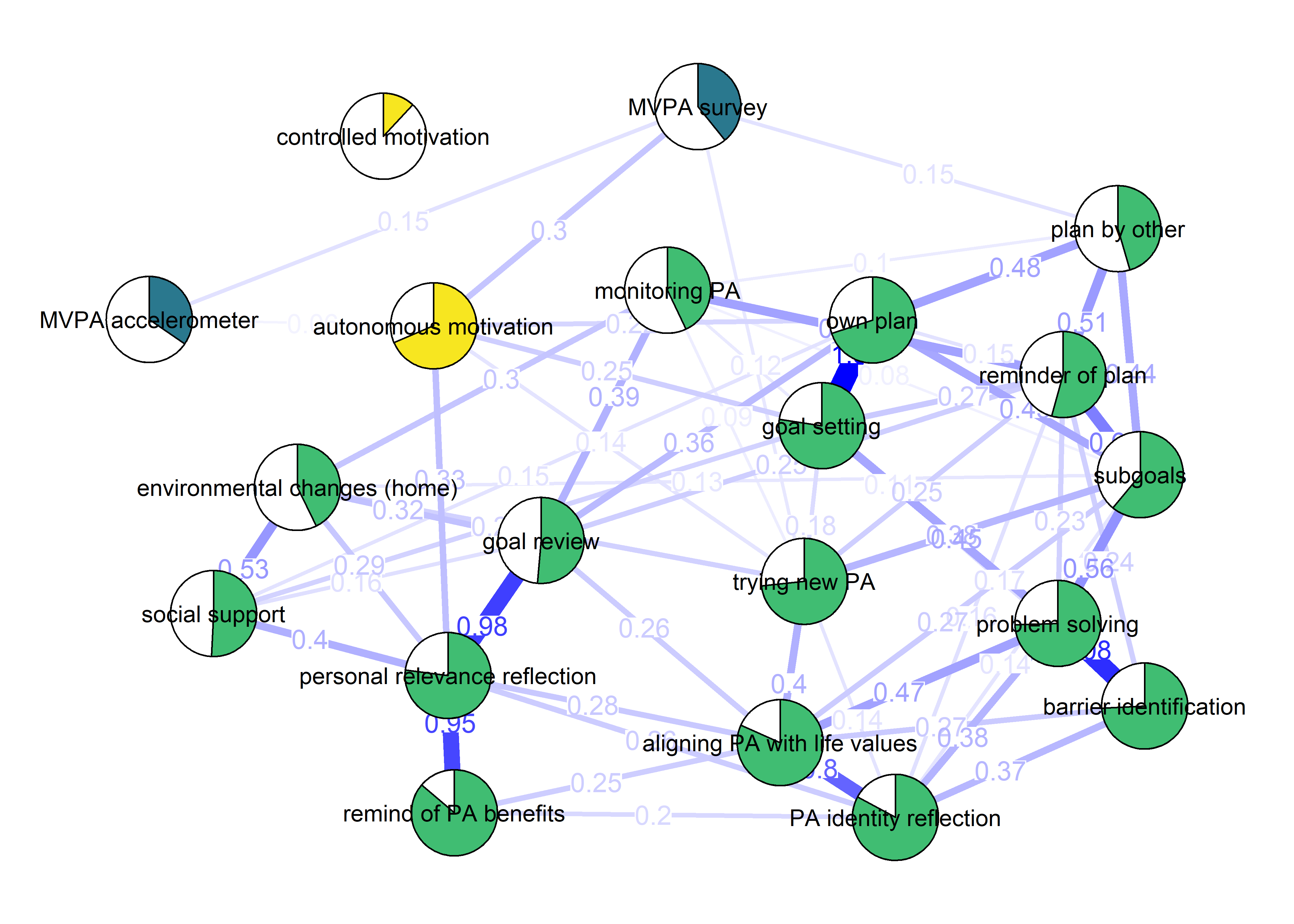
BCT_mgm_T1_circle <- qgraph::qgraph(mgm_obj_T1$pairwise$wadj,
            layout = "circle",
            title = "Mixed graphical model: PA, BCTs & motivation",
            edge.color = ifelse(mgm_obj_T1$pairwise$edgecolor == "darkgreen", "blue", mgm_obj_T1$pairwise$edgecolor),
            pie = pies_T1,
            pieColor = viridis::viridis(5, begin = 0.3, end = 0.8)[5],
            color = node_colors,
            labels = names(bctdf_mgm_T1),
            label.cex = 0.75,
            cut = 0,
            label.scale = FALSE,
            DoNotPlot = TRUE)

plot(BCT_mgm_T1_circle)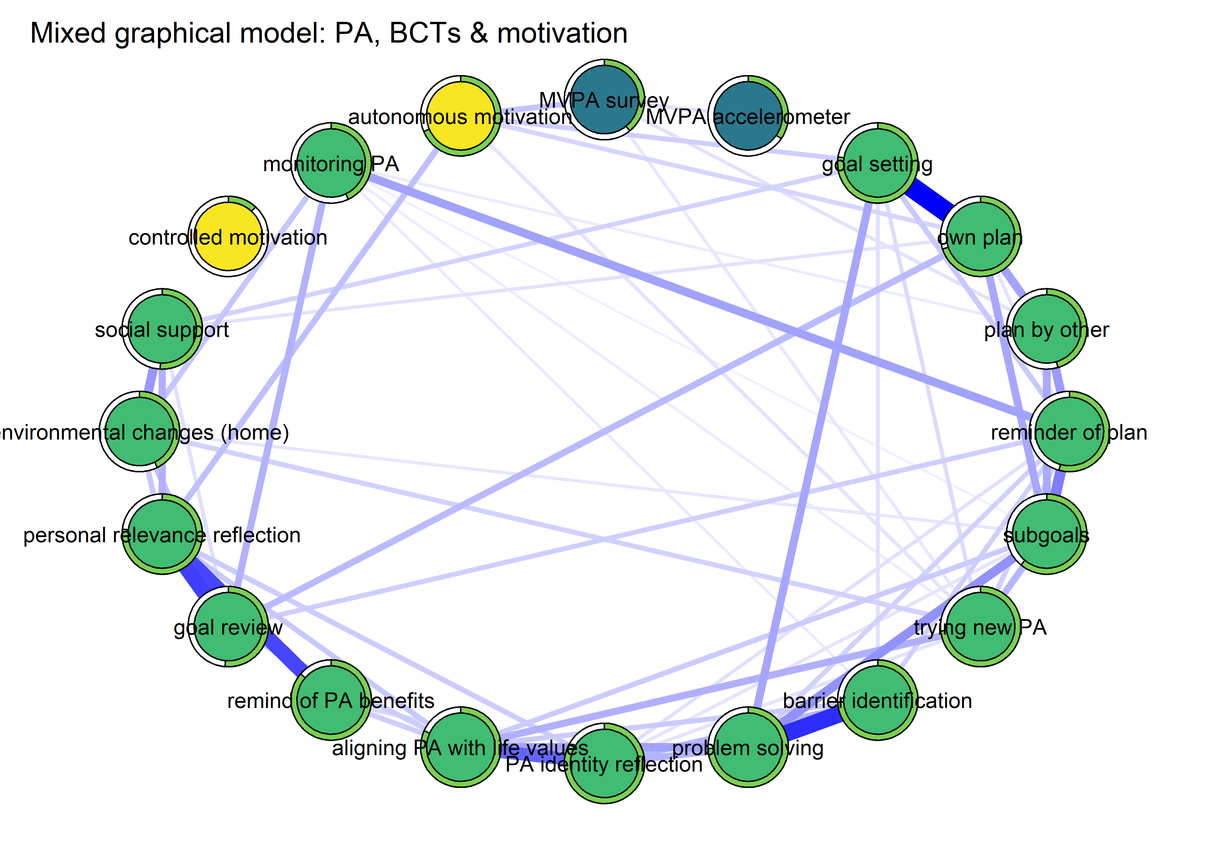
Details and diagnostics
Description
Tabs in this section show robustness diagnostics for the network. For details, see:
Epskamp, S., Borsboom, D., & Fried, E. I. (2018). Estimating psychological networks and their accuracy: A tutorial paper. Behavior Research Methods, 50(1), 195-212. https://doi.org/10.3758/s13428-017-0862-1
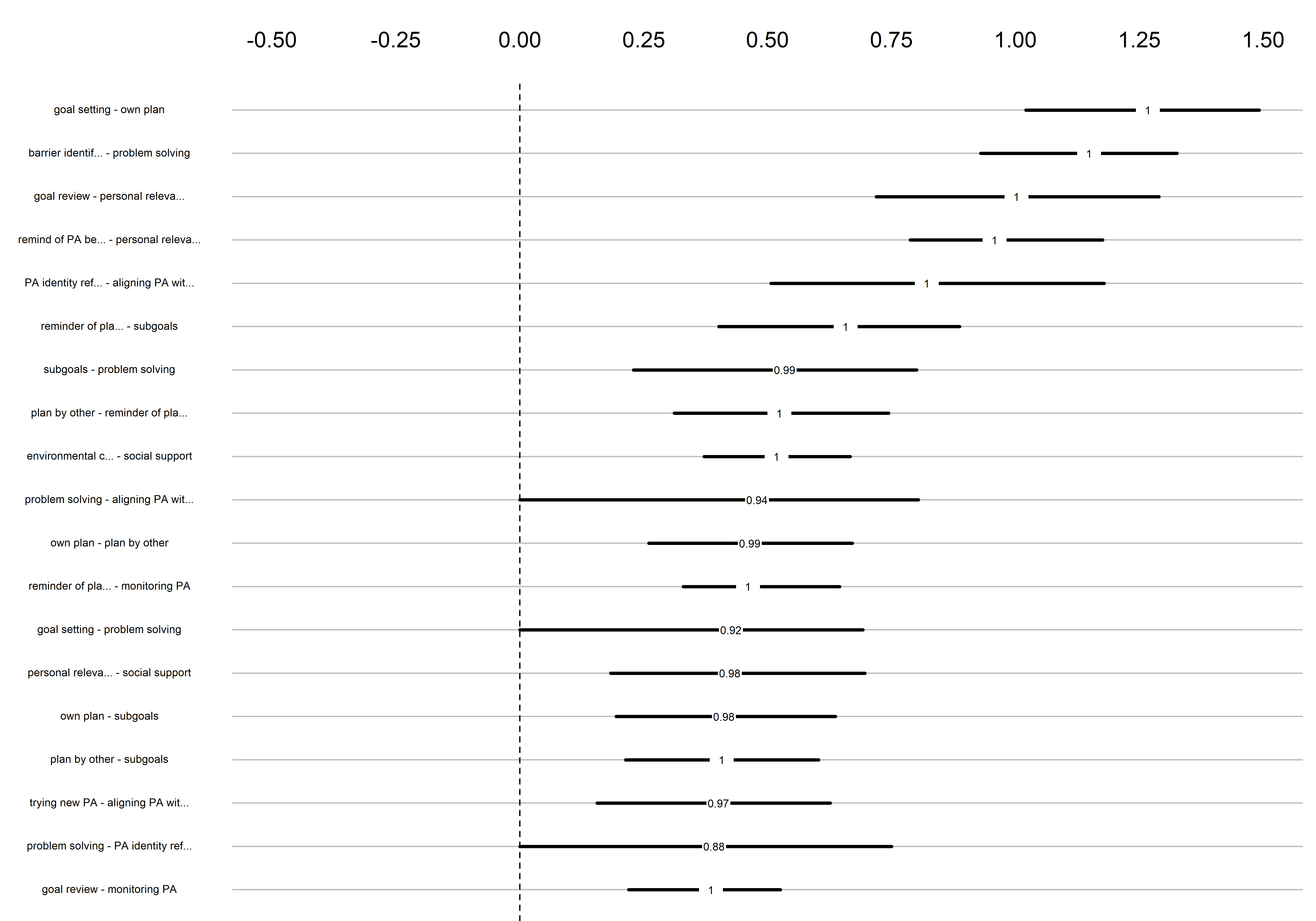
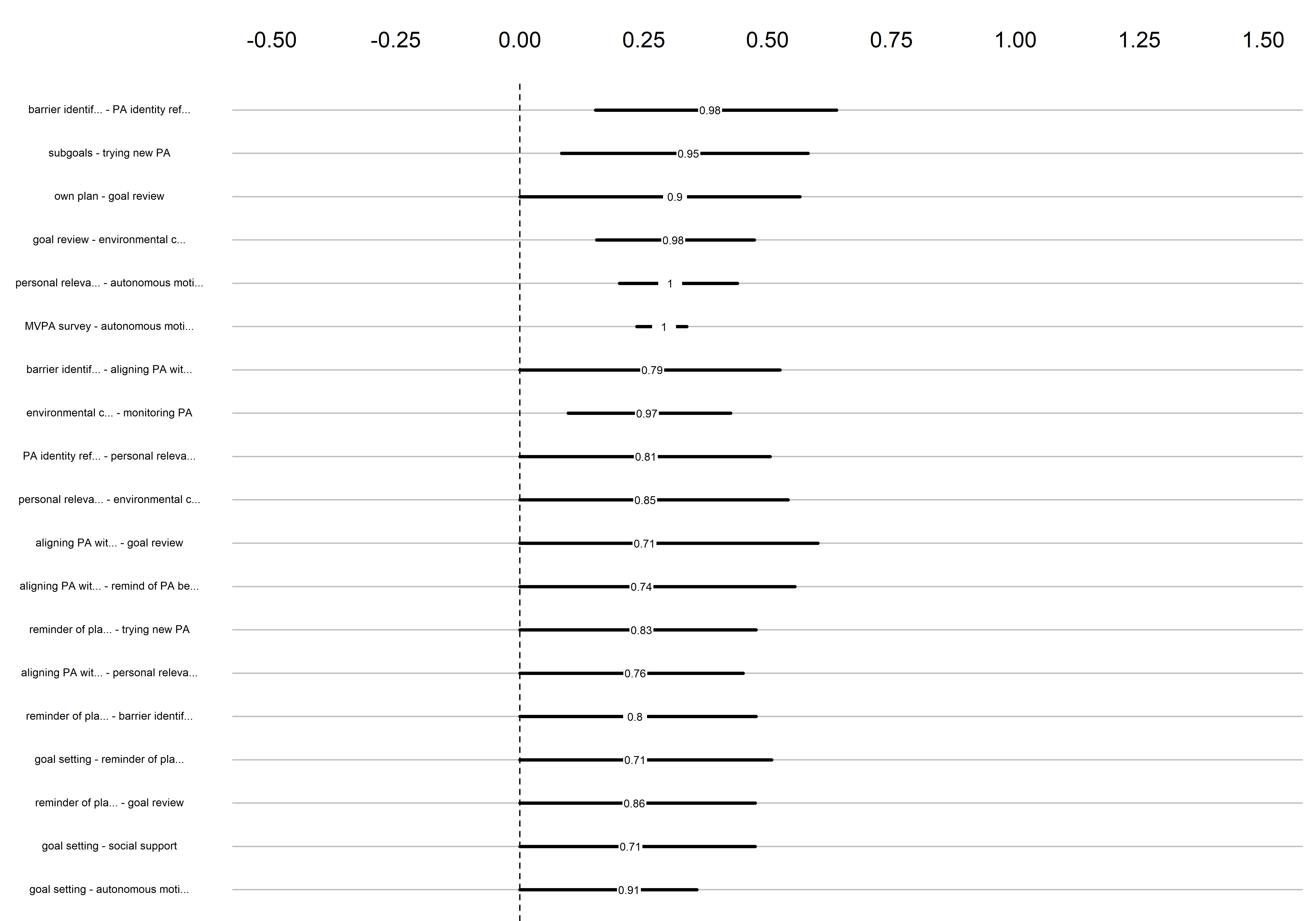
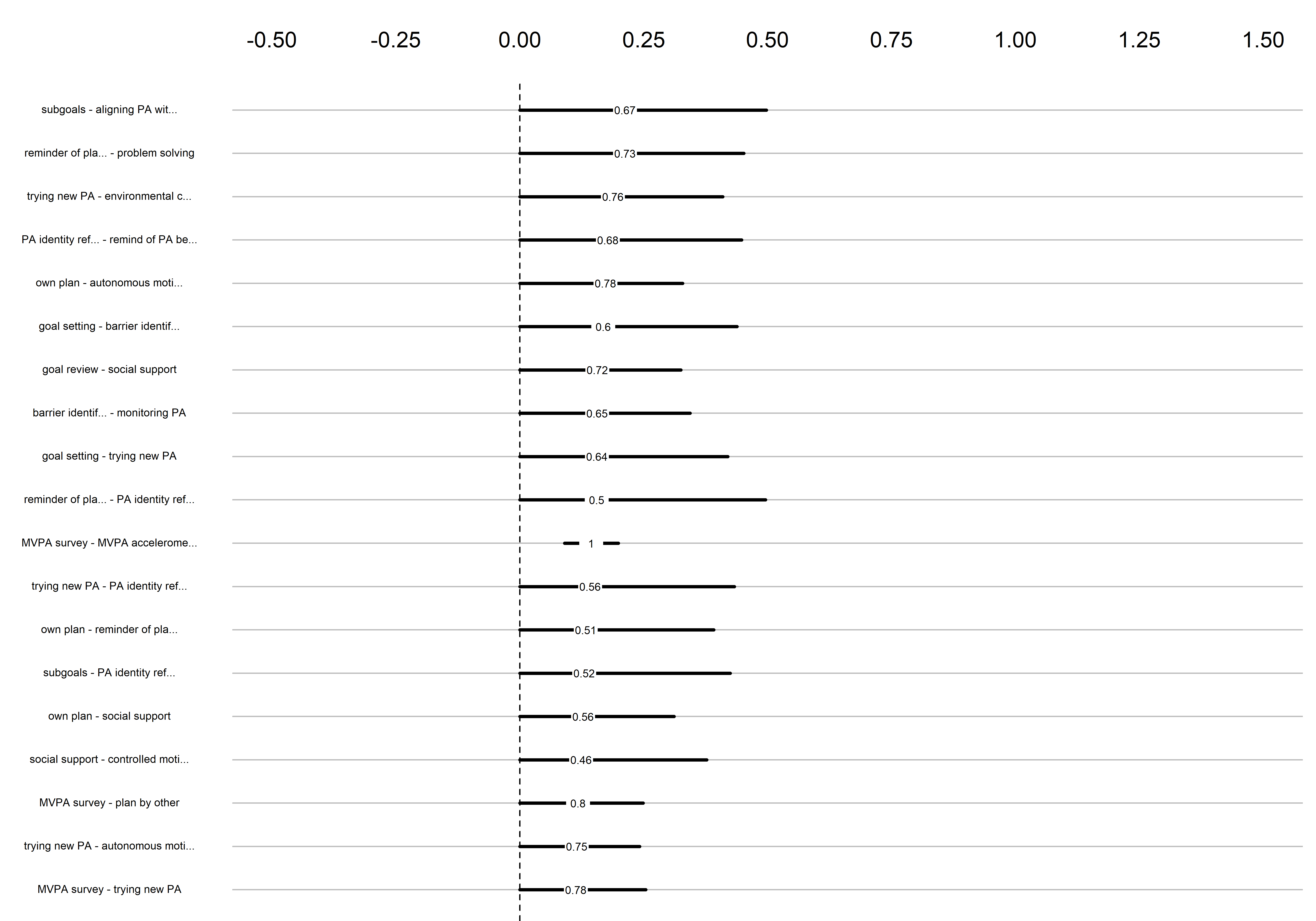
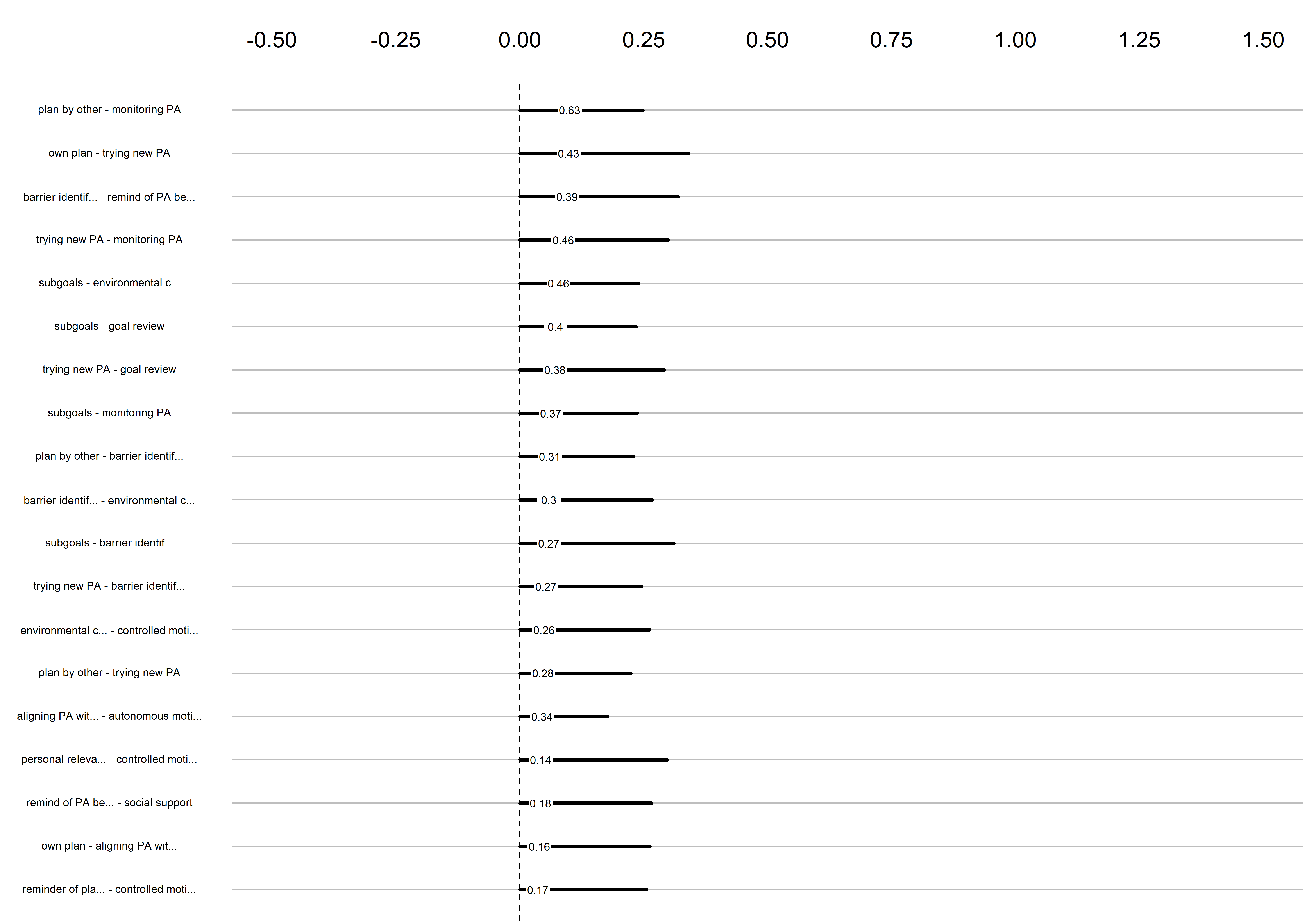
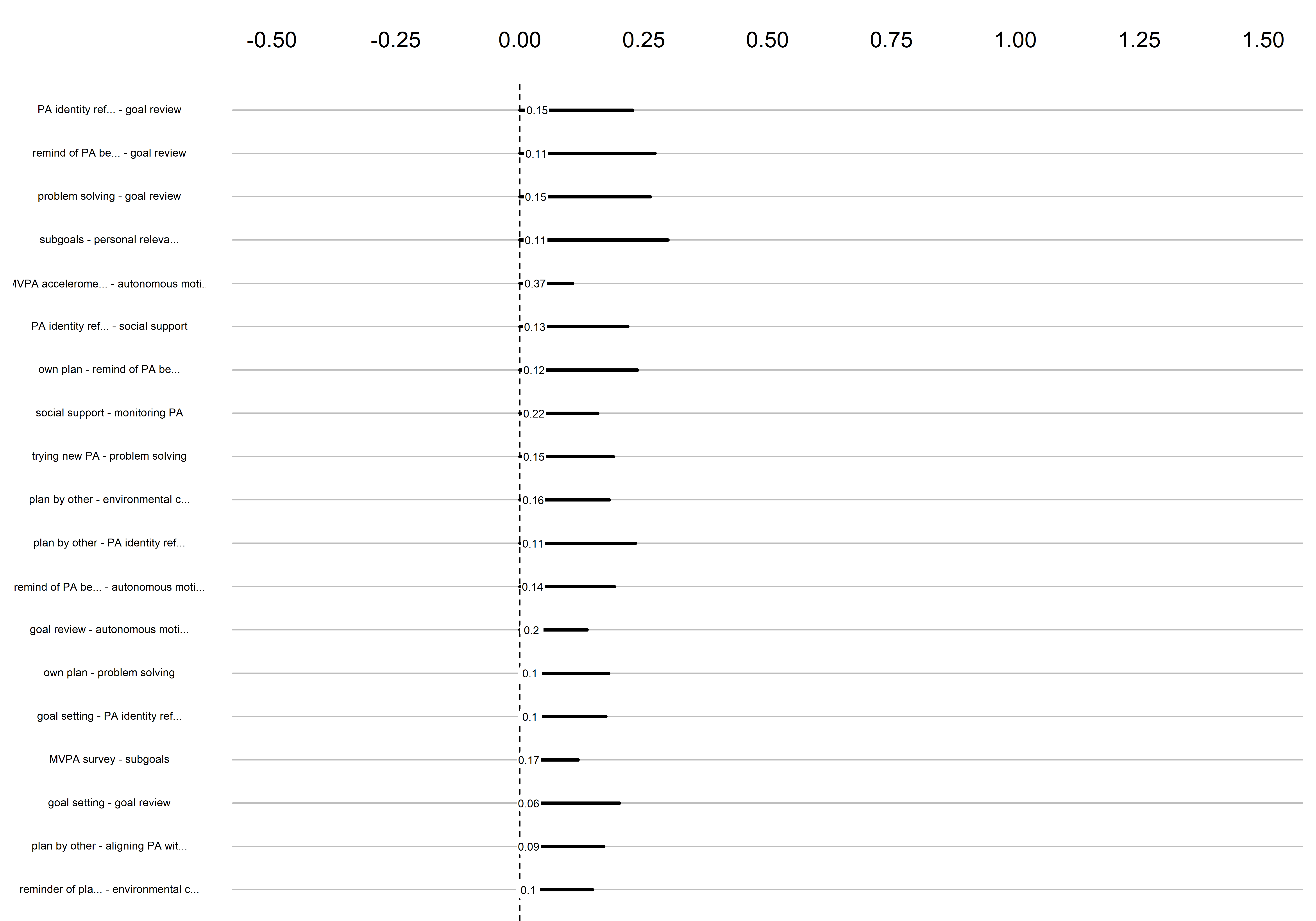
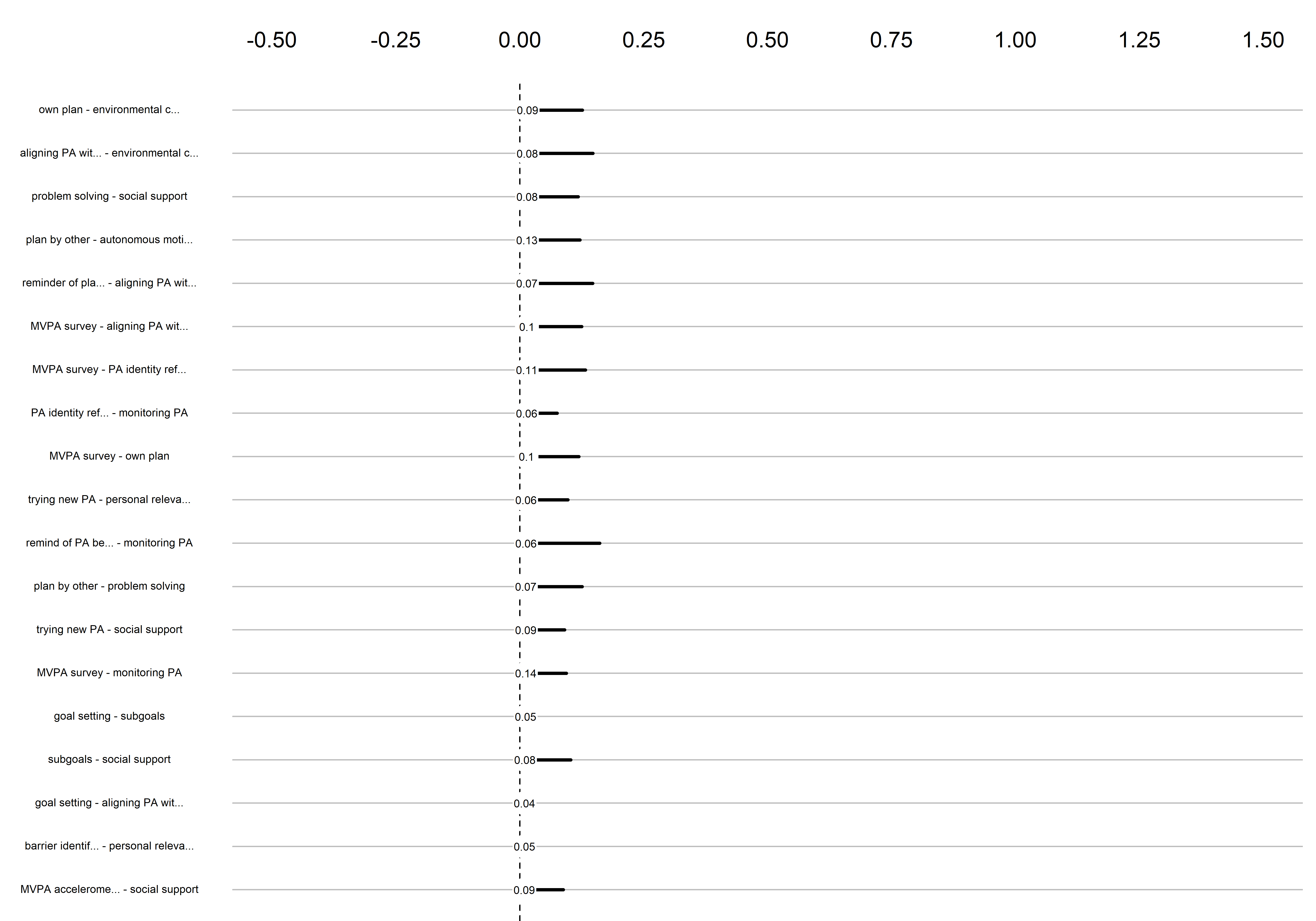
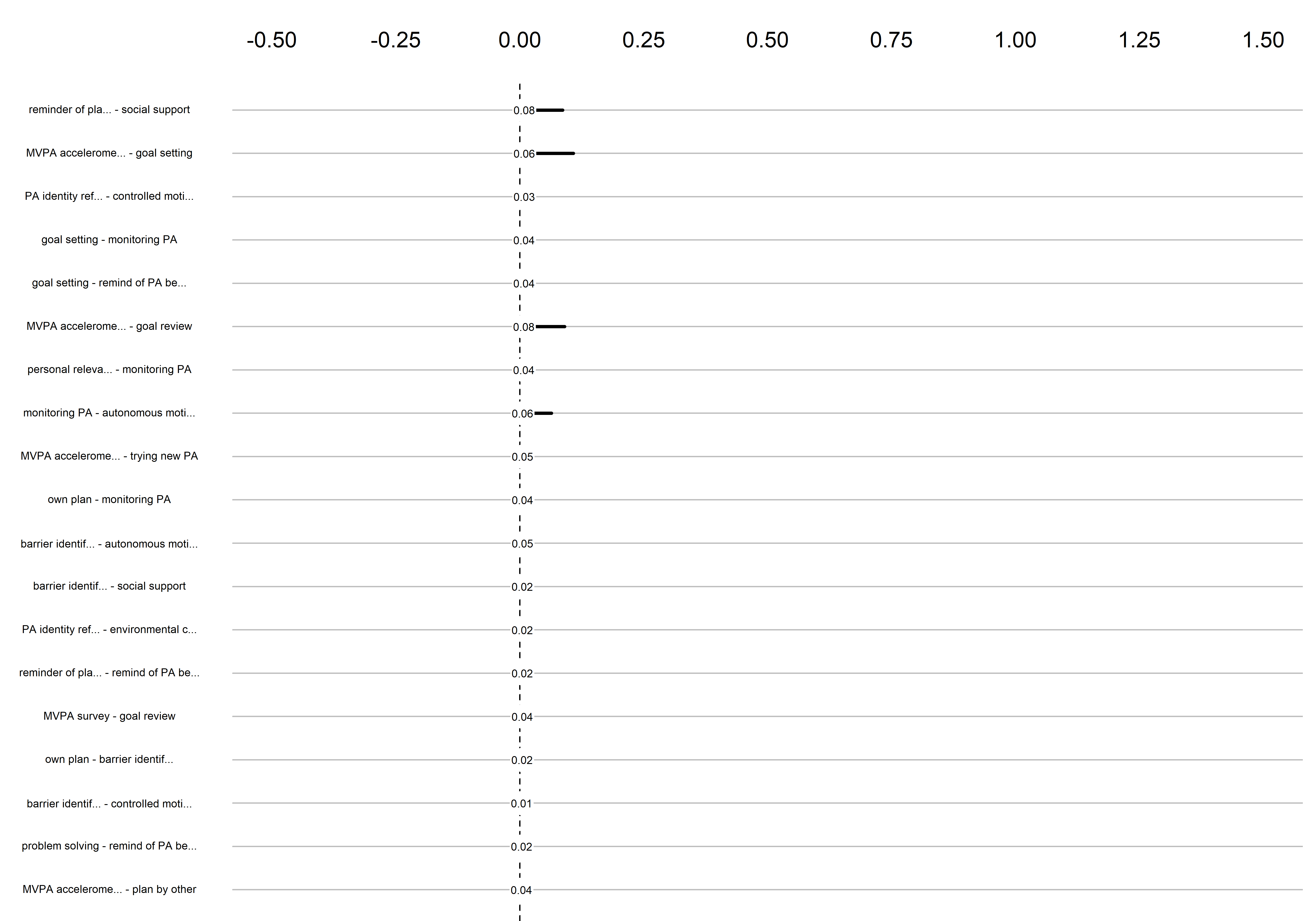
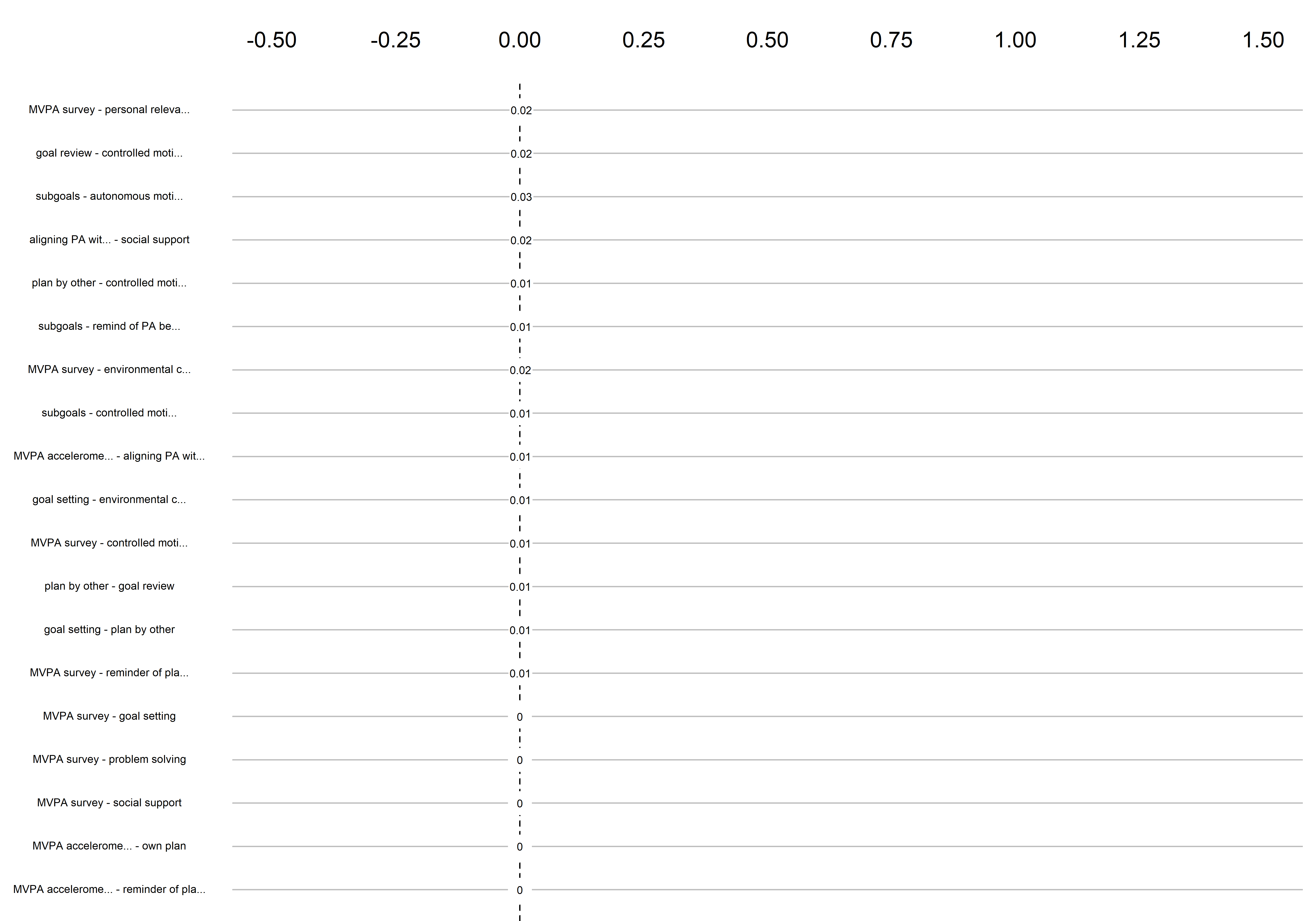
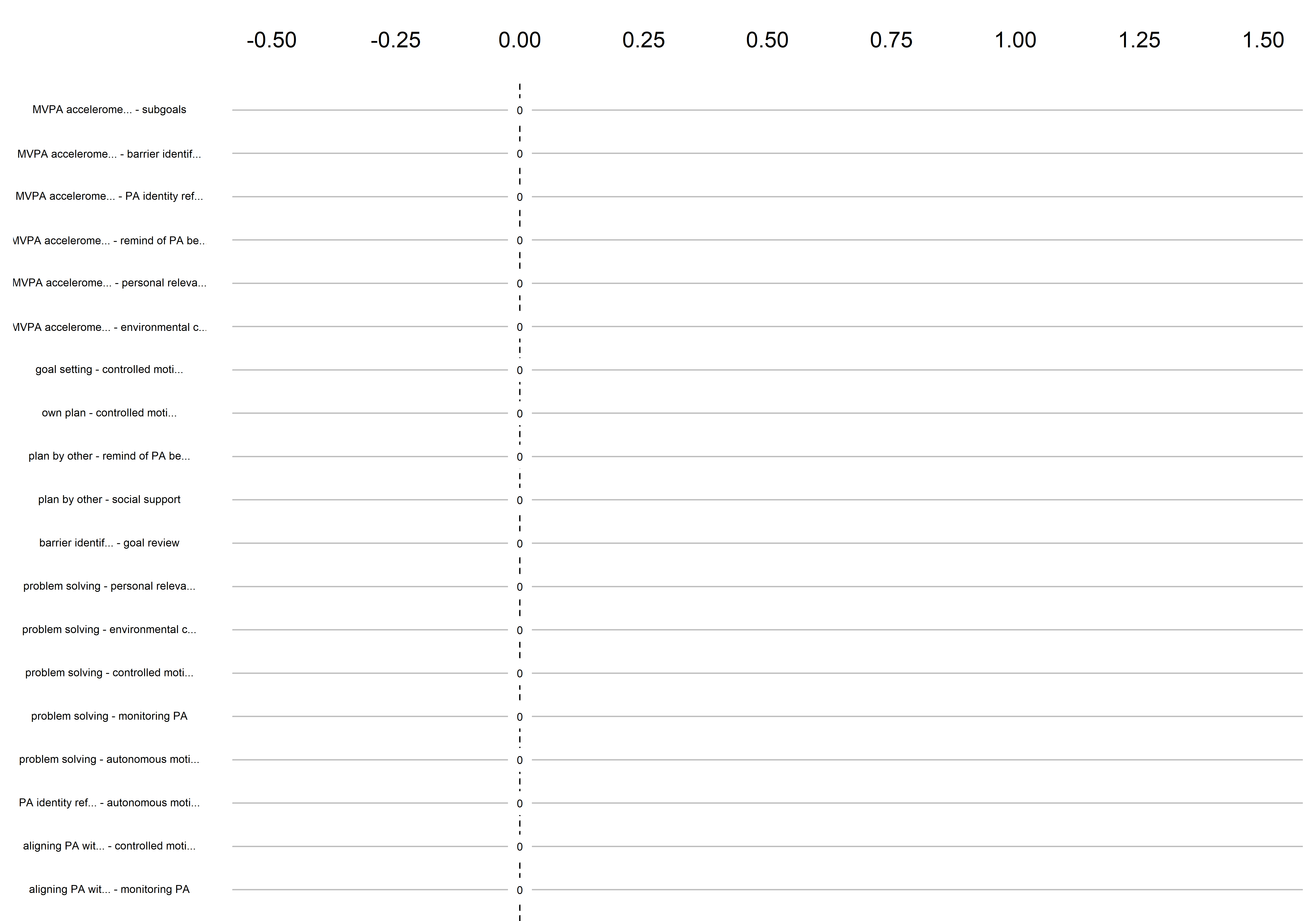
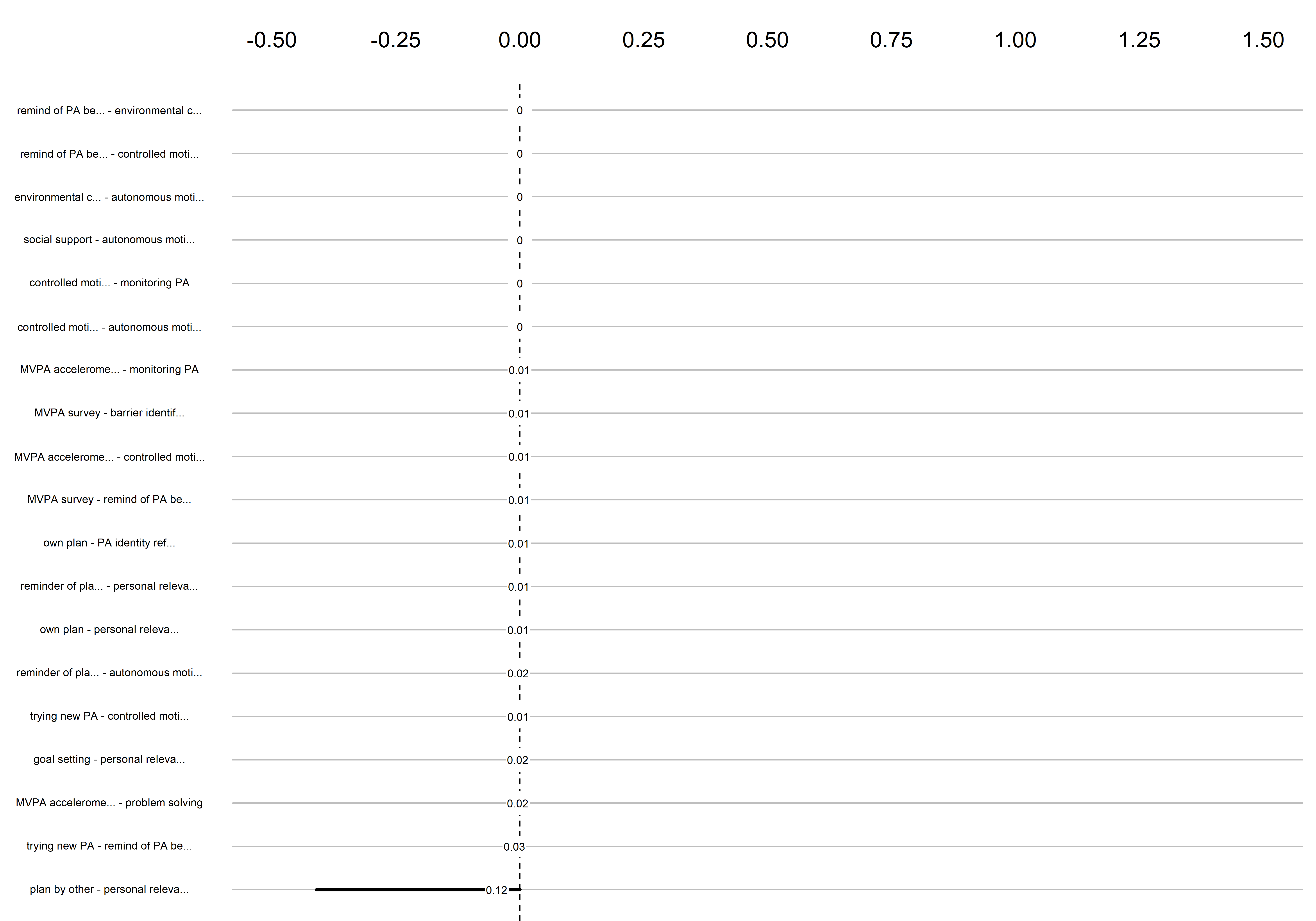
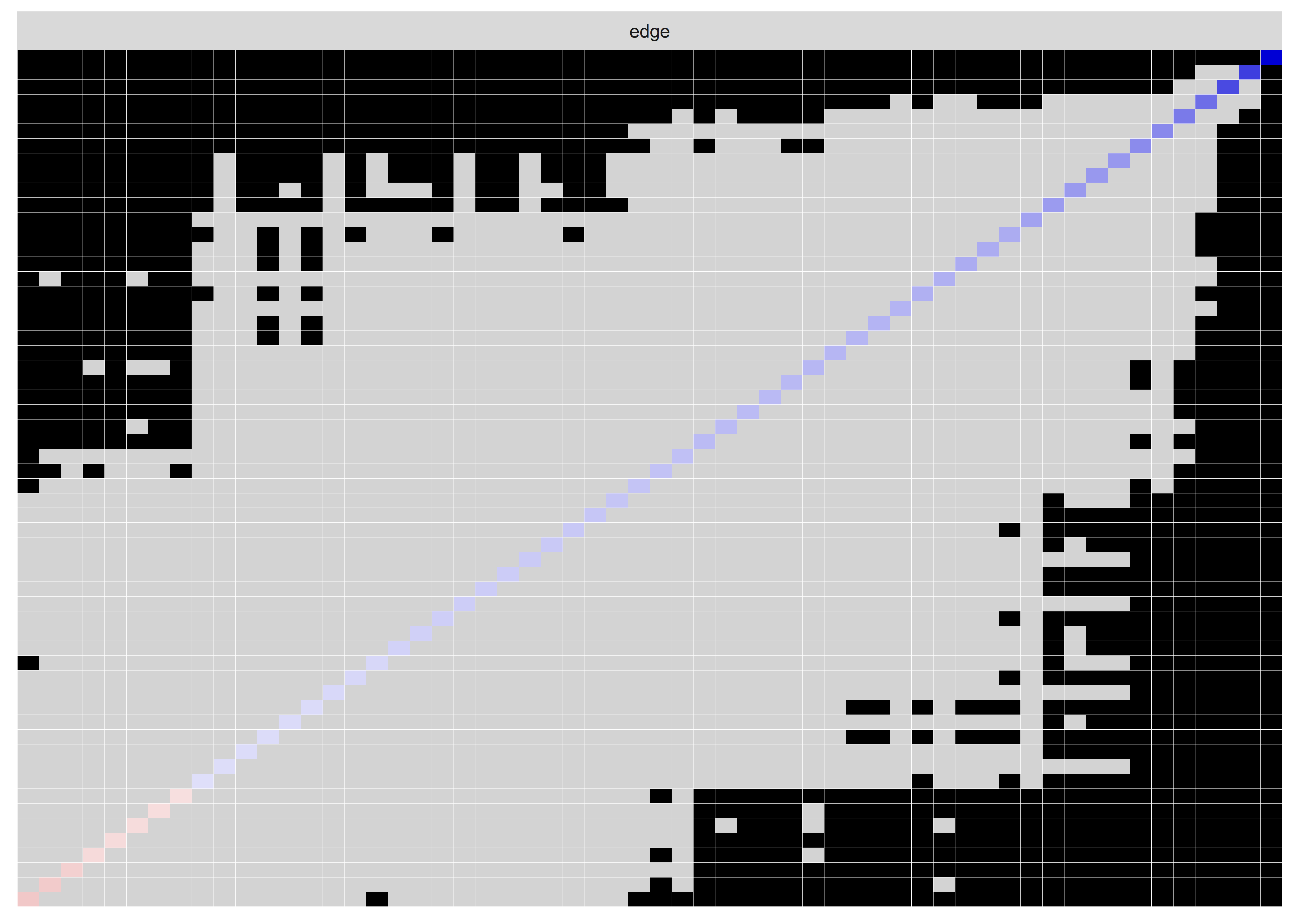
Bootstrap stability
Graphs below depict bootstrapped sampling distributions for the edges, taking 100 bootstrap samples from the original data. Edges are introduced in decreasing order of strength. Line width indicates the edge values drawn from samples between the 5th and 95th quantiles, while the number inside the line is the proportion of non-zero parameter estimates.
# all_BCTs_mgm_stability <- mgm::resample(object = mgm_obj_T1, data = bctdf_mgm_T1, nB = 100)
# save(all_BCTs_mgm_stability, file = "./Rdata_files/all_BCTs_mgm_stability.Rdata")
load("./Rdata_files/all_BCTs_mgm_stability.Rdata")

labels_for_plot <- bctdf_mgm_T1 %>%
  names()

labels_for_plot[nchar(labels_for_plot) > 15] <- paste0(strtrim(labels_for_plot[nchar(labels_for_plot) > 15], 15), "...")

number_of_edges <- ncol(bctdf_mgm_T1) * (ncol(bctdf_mgm_T1) - 1) / 2

for (i in c(seq(from = 1, to = number_of_edges, by = 19))) {

 cat('\n\n####', paste0("edges ", i, "-", i+18), '\n\n  ')

 plot_resample <- mgm::plotRes(object = all_BCTs_mgm_stability,
        quantiles = c(.05, .95),
        cex.label = 0.5,
        lwd.qtl = 2.5,
        cex.mean = .5,
        decreasing = TRUE,
        cut = i:(i+18),
        axis.ticks = c(-0.5, -0.25, 0, 0.25, 0.5, 0.75, 1, 1.25, 1.5),
        labels = labels_for_plot)

 plot_resample
}
edges 1-19
edges 20-38
edges 39-57
edges 58-76
edges 77-95
edges 96-114
edges 115-133
edges 134-152
edges 153-171
edges 172-190
Edge weights matrix
edgeweights <- mgm_obj_T1$pairwise$wadj %>% round(., 3)
colnames(edgeweights) <- labs
rownames(edgeweights) <- labs

edgeweights %>% knitr::kable()| MVPA survey | MVPA accelerometer | goal setting | own plan | plan by other | reminder of plan | subgoals | trying new PA | barrier identification | problem solving | PA identity reflection | aligning PA with life values | remind of PA benefits | goal review | personal relevance reflection | environmental changes (home) | social support | controlled motivation | monitoring PA | autonomous motivation | |
|---|---|---|---|---|---|---|---|---|---|---|---|---|---|---|---|---|---|---|---|---|
| MVPA survey | 0.000 | 0.152 | 0.000 | 0.000 | 0.147 | 0.000 | 0.000 | 0.122 | 0.000 | 0.000 | 0.000 | 0.000 | 0.000 | 0.000 | 0.000 | 0.000 | 0.000 | 0 | 0.000 | 0.299 |
| MVPA accelerometer | 0.152 | 0.000 | 0.000 | 0.000 | 0.000 | 0.000 | 0.000 | 0.000 | 0.000 | 0.000 | 0.000 | 0.000 | 0.000 | 0.000 | 0.000 | 0.000 | 0.000 | 0 | 0.000 | 0.064 |
| goal setting | 0.000 | 0.000 | 0.000 | 1.305 | 0.000 | 0.274 | 0.000 | 0.182 | 0.165 | 0.455 | 0.000 | 0.000 | 0.000 | 0.000 | 0.000 | 0.000 | 0.230 | 0 | 0.000 | 0.250 |
| own plan | 0.000 | 0.000 | 1.305 | 0.000 | 0.477 | 0.146 | 0.449 | 0.000 | 0.000 | 0.000 | 0.000 | 0.000 | 0.000 | 0.356 | 0.000 | 0.000 | 0.147 | 0 | 0.000 | 0.217 |
| plan by other | 0.147 | 0.000 | 0.000 | 0.477 | 0.000 | 0.514 | 0.440 | 0.000 | 0.000 | 0.000 | 0.000 | 0.000 | 0.000 | 0.000 | 0.000 | 0.000 | 0.000 | 0 | 0.100 | 0.000 |
| reminder of plan | 0.000 | 0.000 | 0.274 | 0.146 | 0.514 | 0.000 | 0.659 | 0.250 | 0.245 | 0.233 | 0.159 | 0.000 | 0.000 | 0.249 | 0.000 | 0.000 | 0.000 | 0 | 0.474 | 0.000 |
| subgoals | 0.000 | 0.000 | 0.000 | 0.449 | 0.440 | 0.659 | 0.000 | 0.375 | 0.000 | 0.555 | 0.139 | 0.265 | 0.000 | 0.000 | 0.000 | 0.130 | 0.000 | 0 | 0.079 | 0.000 |
| trying new PA | 0.122 | 0.000 | 0.182 | 0.000 | 0.000 | 0.250 | 0.375 | 0.000 | 0.000 | 0.000 | 0.142 | 0.402 | 0.000 | 0.000 | 0.000 | 0.234 | 0.000 | 0 | 0.093 | 0.138 |
| barrier identification | 0.000 | 0.000 | 0.165 | 0.000 | 0.000 | 0.245 | 0.000 | 0.000 | 0.000 | 1.077 | 0.369 | 0.270 | 0.000 | 0.000 | 0.000 | 0.000 | 0.000 | 0 | 0.111 | 0.000 |
| problem solving | 0.000 | 0.000 | 0.455 | 0.000 | 0.000 | 0.233 | 0.555 | 0.000 | 1.077 | 0.000 | 0.382 | 0.475 | 0.000 | 0.000 | 0.000 | 0.000 | 0.000 | 0 | 0.000 | 0.000 |
| PA identity reflection | 0.000 | 0.000 | 0.000 | 0.000 | 0.000 | 0.159 | 0.139 | 0.142 | 0.369 | 0.382 | 0.000 | 0.796 | 0.198 | 0.000 | 0.259 | 0.000 | 0.000 | 0 | 0.000 | 0.000 |
| aligning PA with life values | 0.000 | 0.000 | 0.000 | 0.000 | 0.000 | 0.000 | 0.265 | 0.402 | 0.270 | 0.475 | 0.796 | 0.000 | 0.254 | 0.261 | 0.279 | 0.000 | 0.000 | 0 | 0.000 | 0.000 |
| remind of PA benefits | 0.000 | 0.000 | 0.000 | 0.000 | 0.000 | 0.000 | 0.000 | 0.000 | 0.000 | 0.000 | 0.198 | 0.254 | 0.000 | 0.000 | 0.948 | 0.000 | 0.000 | 0 | 0.000 | 0.000 |
| goal review | 0.000 | 0.000 | 0.000 | 0.356 | 0.000 | 0.249 | 0.000 | 0.000 | 0.000 | 0.000 | 0.000 | 0.261 | 0.000 | 0.000 | 0.985 | 0.317 | 0.165 | 0 | 0.392 | 0.000 |
| personal relevance reflection | 0.000 | 0.000 | 0.000 | 0.000 | 0.000 | 0.000 | 0.000 | 0.000 | 0.000 | 0.000 | 0.259 | 0.279 | 0.948 | 0.985 | 0.000 | 0.289 | 0.405 | 0 | 0.000 | 0.325 |
| environmental changes (home) | 0.000 | 0.000 | 0.000 | 0.000 | 0.000 | 0.000 | 0.130 | 0.234 | 0.000 | 0.000 | 0.000 | 0.000 | 0.000 | 0.317 | 0.289 | 0.000 | 0.532 | 0 | 0.295 | 0.000 |
| social support | 0.000 | 0.000 | 0.230 | 0.147 | 0.000 | 0.000 | 0.000 | 0.000 | 0.000 | 0.000 | 0.000 | 0.000 | 0.000 | 0.165 | 0.405 | 0.532 | 0.000 | 0 | 0.000 | 0.000 |
| controlled motivation | 0.000 | 0.000 | 0.000 | 0.000 | 0.000 | 0.000 | 0.000 | 0.000 | 0.000 | 0.000 | 0.000 | 0.000 | 0.000 | 0.000 | 0.000 | 0.000 | 0.000 | 0 | 0.000 | 0.000 |
| monitoring PA | 0.000 | 0.000 | 0.000 | 0.000 | 0.100 | 0.474 | 0.079 | 0.093 | 0.111 | 0.000 | 0.000 | 0.000 | 0.000 | 0.392 | 0.000 | 0.295 | 0.000 | 0 | 0.000 | 0.000 |
| autonomous motivation | 0.299 | 0.064 | 0.250 | 0.217 | 0.000 | 0.000 | 0.000 | 0.138 | 0.000 | 0.000 | 0.000 | 0.000 | 0.000 | 0.000 | 0.325 | 0.000 | 0.000 | 0 | 0.000 | 0.000 |
Other estimation methods (mgm CV, GGM)
This section estimates models with different methods: mgm with cross-validation, the standard Gaussian Graphical Model (GGM), and unregularised GGM. The distributions violate normality assumptions of the GGM.
#### CV model selection for mgm

mgm_obj_T1_CV <- mgm::mgm(data = bctdf_mgm_T1,
  type = mgm_variable_types,
  level = mgm_variable_levels,
  lambdaSel = "CV",
  lambdaFolds = 10,
  pbar = FALSE,
  binarySign = TRUE)
## Note that the sign of parameter estimates is stored separately; see ?mgm

# Node pies:
pies_T1 <- bctdf_mgm_T1 %>%
  colMeans() # results in a series of means, which is ok for dichotomous vars
pies_T1["MVPA survey"] <- pies_T1["MVPA survey"] / 7
pies_T1["MVPA accelerometer"] <- pies_T1["MVPA accelerometer"] / max(bctdf_mgm_T1$`MVPA accelerometer`, na.rm = TRUE)
pies_T1["autonomous motivation"] <- pies_T1["autonomous motivation"] / 5


node_colors <- c(viridis::viridis(3, begin = 0.4, end = 0.99)[1], # Color 1 for MVPA (questionnaire)
                 viridis::viridis(3, begin = 0.4, end = 0.99)[1], # Color 1 for MVPA (accelerometer)
                 rep(viridis::viridis(3, begin = 0.4, end = 0.99)[2], 15), # 11x Color 2 for BCTs
                 rep(viridis::viridis(3, begin = 0.4, end = 0.99)[3], 1), # Color 3 for motivation (controlled)
                 rep(viridis::viridis(3, begin = 0.4, end = 0.99)[2], 1), # 1x Color 2 for BCTs
                 viridis::viridis(3, begin = 0.4, end = 0.99)[3]) # Color 3 for motivation (autonomous)

BCT_mgm_T1_CV <- qgraph::qgraph(mgm_obj_T1_CV$pairwise$wadj,
            layout = BCT_mgm_T1$layout,
            repulsion = 0.99, # To nudge the network from originally bad visual state
            edge.color = ifelse(mgm_obj_T1$pairwise$edgecolor == "darkgreen", "blue", mgm_obj_T1$pairwise$edgecolor),
            pie = pies_T1,
            # pieColor = pie_colors_T1,
            pieColor = node_colors,
            labels = names(bctdf_mgm_T1),
            pieBorder = 1,
            label.cex = 0.75,
            cut = 0,
            label.scale = FALSE,
            title = "MGM with cross-validation")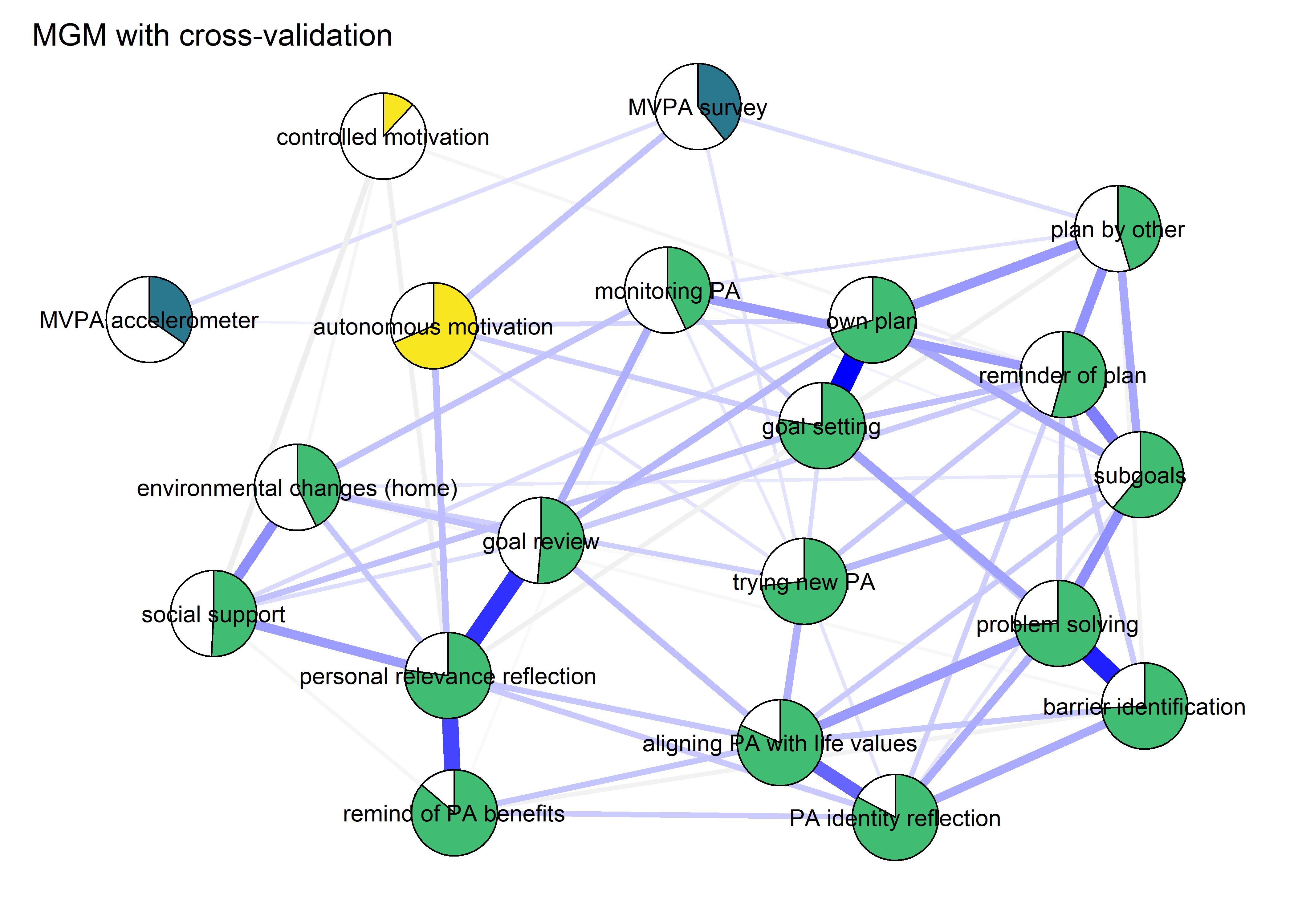
#### GGM
bctdf_ggm_T1 <- df %>% dplyr::select(
'goal setting' = PA_agreementDependentBCT_01_T1,
'own plan' = PA_agreementDependentBCT_02_T1,
'plan by other' = PA_agreementDependentBCT_03_T1,
'reminder of plan' = PA_agreementDependentBCT_04_T1,
'subgoals' = PA_agreementDependentBCT_05_T1,
'trying new PA' = PA_agreementDependentBCT_06_T1,
'barrier identification' = PA_agreementDependentBCT_07_T1,
'problem solving' = PA_agreementDependentBCT_08_T1,
'PA identity reflection' = PA_agreementDependentBCT_09_T1,
'aligning PA with life values' = PA_agreementDependentBCT_10_T1,
'remind of PA benefits' = PA_frequencyDependentBCT_01_T1,
'self-monitor (paper)' = PA_frequencyDependentBCT_02_T1,
'self-monitor (app)' = PA_frequencyDependentBCT_03_T1,
# 'memory cues' = PA_frequencyDependentBCT_04_T1, # Issues with clarity of item wording
'goal review' = PA_frequencyDependentBCT_05_T1,
'personal relevance reflection' = PA_frequencyDependentBCT_06_T1,
'environmental changes (home)' = PA_frequencyDependentBCT_07_T1,
'social support' = PA_frequencyDependentBCT_08_T1,
'analysing goal failure' = PA_frequencyDependentBCT_09_T1,
'MVPA survey' = padaysLastweek_T1,
'MVPA accelerometer' = mvpaAccelerometer_T1,
'intrinsic' = PA_intrinsic_T1,
'identified' = PA_identified_T1, 'integrated' = PA_integrated_T1,
'controlled motivation' = PA_controlled_T1) %>%
rowwise() %>%
mutate(
# 'goal setting' = ifelse(`goal setting` == 1, 0, 1),
# 'own plan' = ifelse(`own plan` == 1, 0, 1),
# 'plan by other' = ifelse(`plan by other` == 1, 0, 1),
# 'reminder of plan' = ifelse(`reminder of plan` == 1, 0, 1),
# 'subgoals' = ifelse(`subgoals` == 1, 0, 1),
# 'trying new PA' = ifelse(`trying new PA` == 1, 0, 1),
# 'barrier identification' = ifelse(`barrier identification` == 1, 0, 1),
# 'problem solving' = ifelse(`problem solving` == 1, 0, 1),
# 'PA identity reflection' = ifelse(`PA identity reflection` == 1, 0, 1),
# 'aligning PA with life values' = ifelse(`aligning PA with life values` == 1, 0, 1),
# 'remind of PA benefits' = ifelse(`remind of PA benefits` == 1, 0, 1),
'monitoring PA' = ifelse(`self-monitor (paper)` == 1 & `self-monitor (app)` == 1, 0, 1),
# 'goal review' = ifelse(`goal review` == 1, 0, 1),
# 'personal relevance reflection' = ifelse(`personal relevance reflection` == 1, 0, 1),
# 'environmental changes (home)' = ifelse(`environmental changes (home)` == 1, 0, 1),
# 'social support' = ifelse(`social support` == 1, 0, 1),
# 'analysing goal failure' = ifelse(`analysing goal failure` == 1, 0, 1),
'autonomous motivation' = mean(c(identified, intrinsic, integrated), na.rm = T),
'controlled motivation' = `controlled motivation` * 1) %>%
dplyr::select(-`self-monitor (paper)`, -`self-monitor (app)`,
-identified, -intrinsic, -integrated,
-`analysing goal failure` # only concerns those who haven't reached goals
) %>%
dplyr::select('MVPA survey', 'MVPA accelerometer', everything()) %>%
mutate_all(as.numeric)
nwBCT_ggm <- bootnet::estimateNetwork(bctdf_ggm_T1, default="ggmModSelect")
BCT_ggm <- plot(nwBCT_ggm,
layout = BCT_mgm_T1$layout,
label.scale = FALSE,
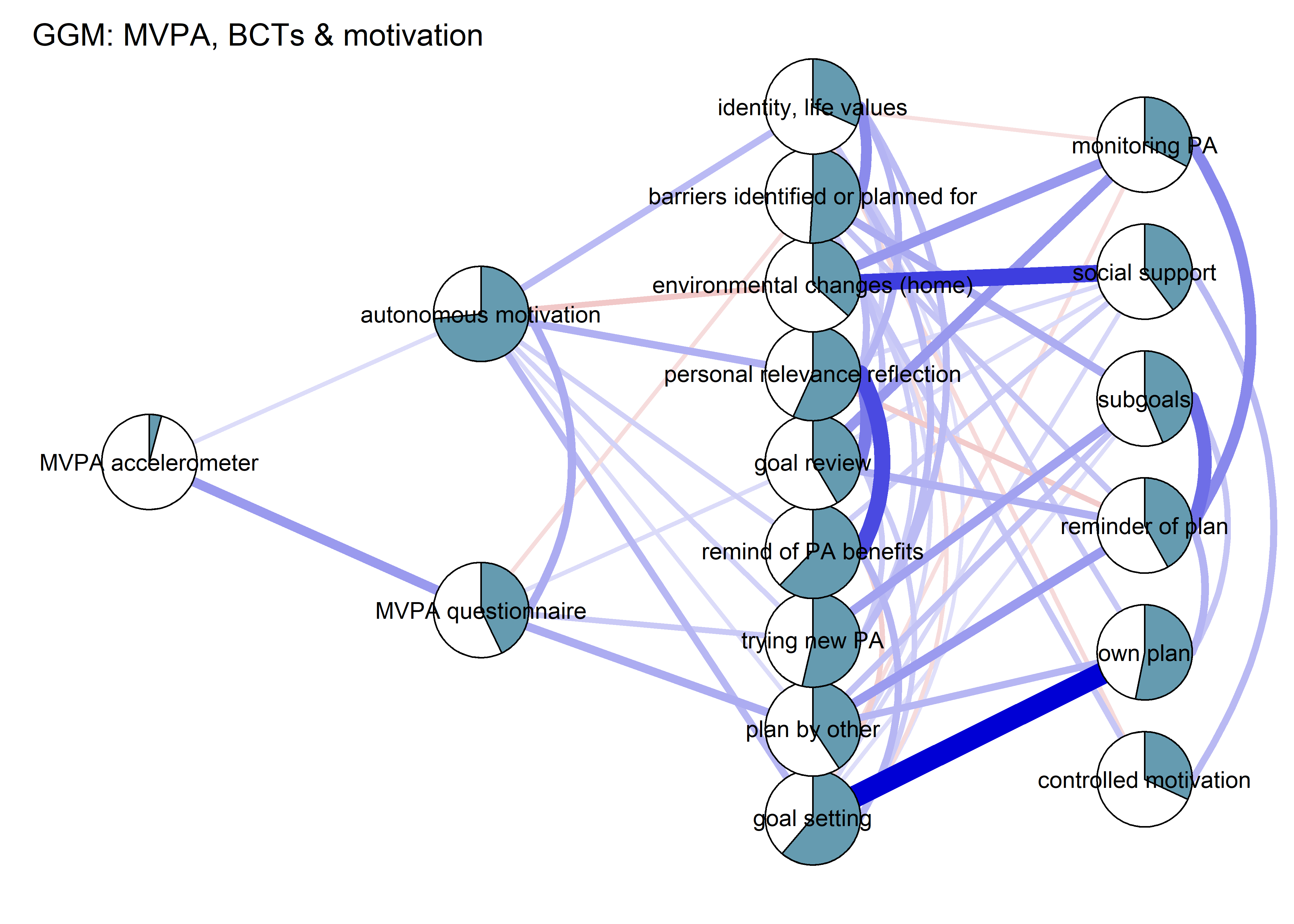
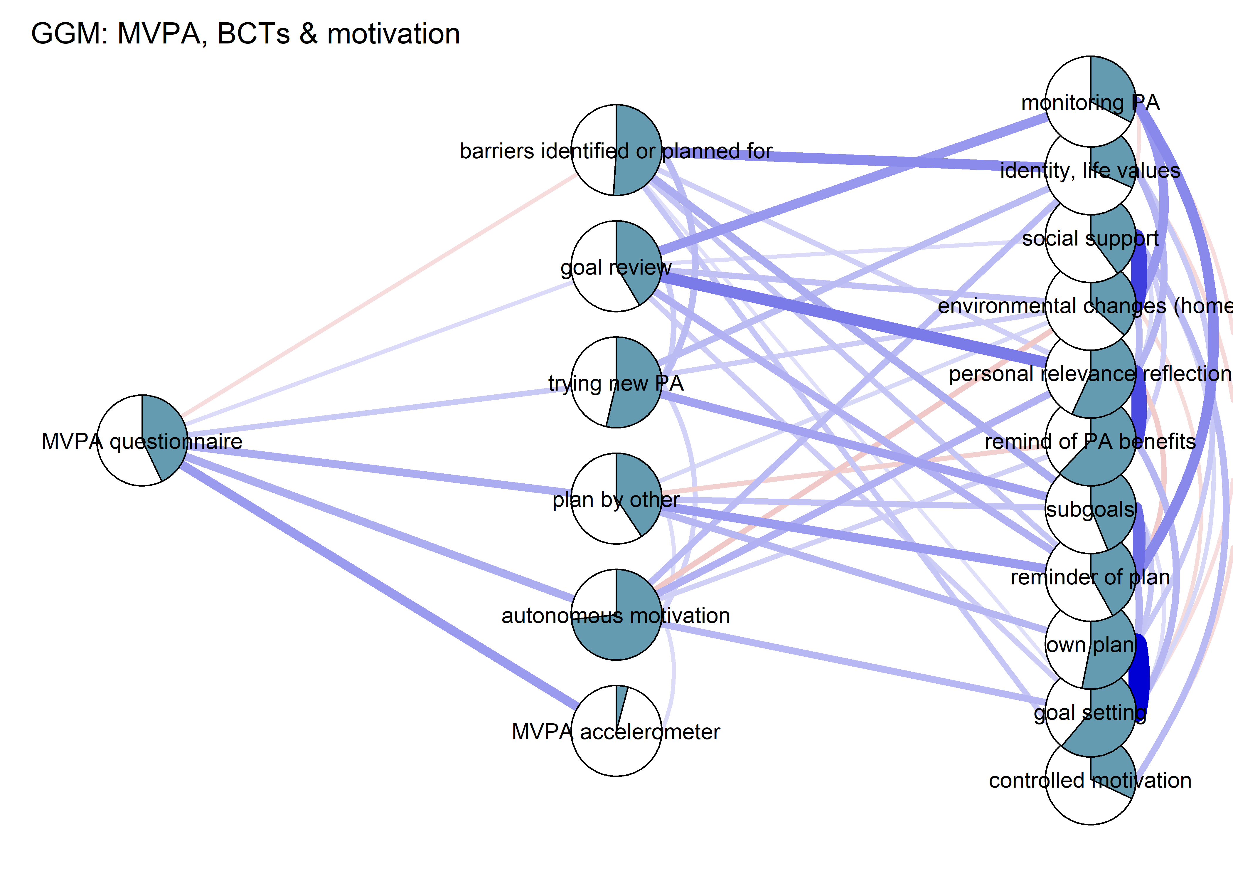
title = "GGM: MVPA, BCTs & motivation",
label.cex = 0.75,
# pie = piefill_ggm,
color = node_colors,
pieBorder = 1)
modSelect_0 <- qgraph::ggmModSelect(qgraph::cor_auto(bctdf_ggm_T1), n = nrow(bctdf_ggm_T1), gamma = 0)

g3 <- qgraph::qgraph(modSelect_0$graph,
                     layout = BCT_mgm_T1$layout,
                     label.scale = FALSE,
                     label.cex = 0.75,
                     labels = labs,
                     theme = "colorblind",
                     title = "ggmModSelect (gamma = 0)",
                     color = node_colors,
                     cut = 0)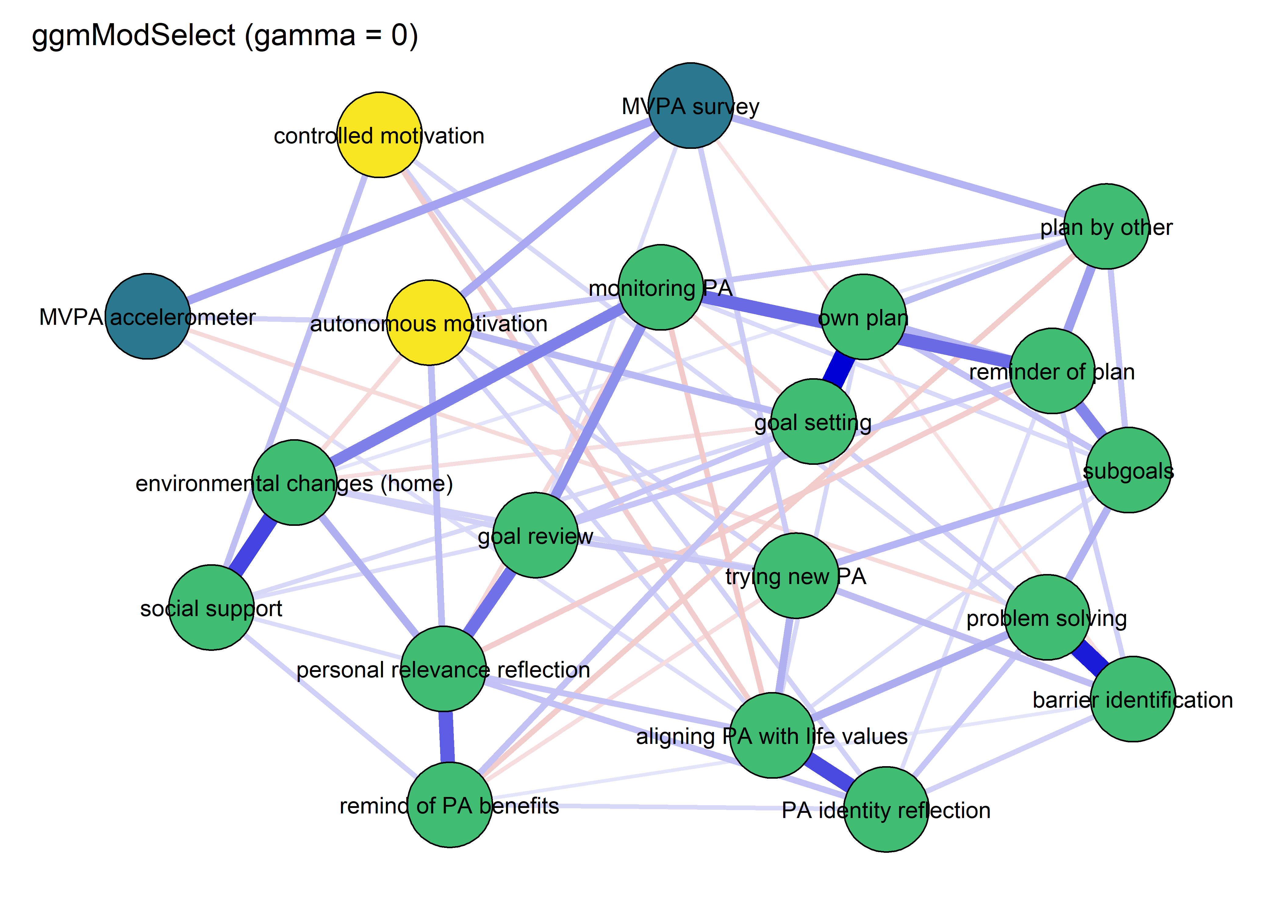
modSelect_0.5 <- qgraph::ggmModSelect(qgraph::cor_auto(bctdf_ggm_T1), n = nrow(bctdf_ggm_T1), gamma = 0.5)

g4 <- qgraph::qgraph(modSelect_0.5$graph,
                     layout = BCT_mgm_T1$layout,
                     label.scale = FALSE,
                     label.cex = 0.75,
                     labels = labs,
                     theme = "colorblind",
                     title = "ggmModSelect (gamma = 0.5)",
                     color = node_colors,
                     cut = 0)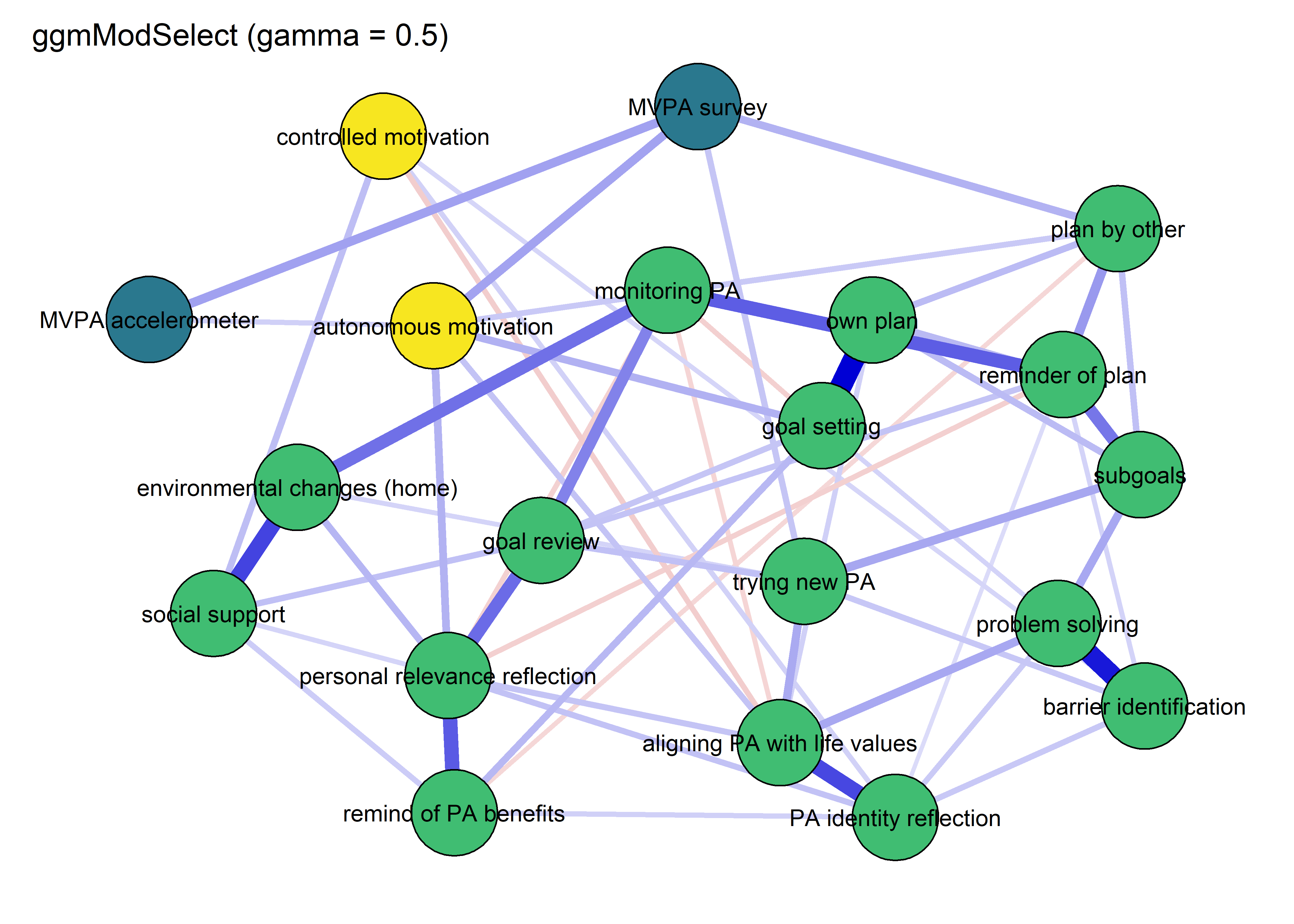
Autonomous motivation as moderator
Moderation analysis with mgm did not indicate autonomous motivation as a moderator for any edges. This may be due to lack of statistical power (or specificity), lack of a true effect, or e.g. the process taking place within and not between individuals.
bctdf_mgm_T1 <- df %>% dplyr::select(
#  id,
#  intervention,
#  group,
#  school,
#  girl,
  'goal setting' = PA_agreementDependentBCT_01_T1,
  'own plan' = PA_agreementDependentBCT_02_T1,
  'plan by other' = PA_agreementDependentBCT_03_T1,
  'reminder of plan' = PA_agreementDependentBCT_04_T1,
  'subgoals' = PA_agreementDependentBCT_05_T1,
  'trying new PA' = PA_agreementDependentBCT_06_T1,
  'barrier identification' = PA_agreementDependentBCT_07_T1,
  'problem solving' = PA_agreementDependentBCT_08_T1,
  'PA identity reflection' = PA_agreementDependentBCT_09_T1,
  'aligning PA with life values' = PA_agreementDependentBCT_10_T1,
  'remind of PA benefits' = PA_frequencyDependentBCT_01_T1,
  'self-monitor (paper)' = PA_frequencyDependentBCT_02_T1,
  'self-monitor (app)' = PA_frequencyDependentBCT_03_T1,
#  'memory cues' = PA_frequencyDependentBCT_04_T1, # Issues with clarity of item wording
  'goal review' = PA_frequencyDependentBCT_05_T1,
  'personal relevance reflection' = PA_frequencyDependentBCT_06_T1,
  'environmental changes (home)' = PA_frequencyDependentBCT_07_T1,
  'social support' = PA_frequencyDependentBCT_08_T1,
  'analysing goal failure' = PA_frequencyDependentBCT_09_T1,
  'MVPA survey' = padaysLastweek_T1,
  'MVPA accelerometer' = mvpaAccelerometer_T1,
  'intrinsic' = PA_intrinsic_T1,
  'identified' = PA_identified_T1, 'integrated' = PA_integrated_T1,
  'controlled motivation' = PA_controlled_T1) %>%
 rowwise() %>%
 mutate(
  'goal setting' = ifelse(`goal setting` == 1, 0, 1),
#  'has plan' = ifelse(`own plan` == 1 & `plan by other` == 1, 0, 1),
  'own plan' = ifelse(`own plan` == 1, 0, 1),
  'plan by other' = ifelse(`plan by other` == 1, 0, 1),
  'reminder of plan' = ifelse(`reminder of plan` == 1, 0, 1),
  'subgoals' = ifelse(`subgoals` == 1, 0, 1),
  'trying new PA' = ifelse(`trying new PA` == 1, 0, 1),
  'barrier identification' = ifelse(`barrier identification` == 1, 0, 1),
  'problem solving' = ifelse(`problem solving` == 1, 0, 1),
  # 'barriers identified or planned for' = ifelse(`problem solving` == 1 & `barrier identification` == 1, 0, 1),
  'PA identity reflection' = ifelse(`PA identity reflection` == 1, 0, 1),
  'aligning PA with life values' = ifelse(`aligning PA with life values` == 1, 0, 1),
  # 'identity, life values' = ifelse(`PA identity reflection` == 1 & `aligning PA with life values` == 1, 0, 1),
  'remind of PA benefits' = ifelse(`remind of PA benefits` == 1, 0, 1),
  'monitoring PA' = ifelse(`self-monitor (paper)` == 1 & `self-monitor (app)` == 1, 0, 1),
#  'memory cues' = ifelse(`memory cues` == 1, 0, 1),
  'goal review' = ifelse(`goal review` == 1, 0, 1),
  'personal relevance reflection' = ifelse(`personal relevance reflection` == 1, 0, 1),
  'environmental changes (home)' = ifelse(`environmental changes (home)` == 1, 0, 1),
  'social support' = ifelse(`social support` == 1, 0, 1),
  'analysing goal failure' = ifelse(`analysing goal failure` == 1, 0, 1),
  'autonomous motivation' = mean(c(identified, intrinsic, integrated), na.rm = T),
#  'girl' = ifelse(girl == "girl", 1, 0),
  'controlled motivation' = ifelse(`controlled motivation` < 3, 0, 1)) %>%  # If "at least partly" or more true, input 1. Normality otherwise a problem.
#  'intervention' = ifelse(intervention == "1", 1, 0)) %>%
  dplyr::select(-`self-monitor (paper)`, -`self-monitor (app)`,
                # -`plan by other`, -`own plan`,
                -identified, -intrinsic, -integrated,
         -`analysing goal failure` # only concerns those who haven't reached goals
         # -`barrier identification`, -`problem solving`, # closely related
           ) %>%
#  dplyr::select(-controlled) %>% # Not really gaussian at all
  dplyr::select('MVPA survey', 'MVPA accelerometer', everything())

bctdf_mgm_T1$`autonomous motivation`[is.nan(bctdf_mgm_T1$`autonomous motivation`)] <- NA

labs <- names(bctdf_mgm_T1)

# mgm wants full data, see package missForest for imputation methods
bctdf_mgm_T1 <- bctdf_mgm_T1 %>% na.omit(.)
# bctdf_mgm %>% names()
mgm_variable_types <- c("g", "g", rep("c", 17), "g")
mgm_variable_levels <- c("1", "1", rep("2", 17), "1")
# data.frame(mgm_variable_types, mgm_variable_levels, names(bctdf_mgm))

mgm_obj_T1_moderated <- mgm::mgm(data = bctdf_mgm_T1,
  type = mgm_variable_types,
  level = mgm_variable_levels,
  lambdaSel = "EBIC",
  # lambdaFolds = 10,
  moderators = 20,
  verbatim = FALSE,
  pbar = FALSE,
  binarySign = TRUE)
## Note that the sign of parameter estimates is stored separately; see ?mgm

mgm::FactorGraph(object = mgm_obj_T1_moderated,
                 # pie = pies_T1,
                 # pieColor = pie_colors_T1,
                 # pieColor = node_colors,
                 pieBorder = 1,
                 label.cex = 0.85,
                 PairwiseAsEdge = TRUE,
                 edge.labels = TRUE,
                 label.scale = FALSE,
                 labels = names(bctdf_mgm_T1))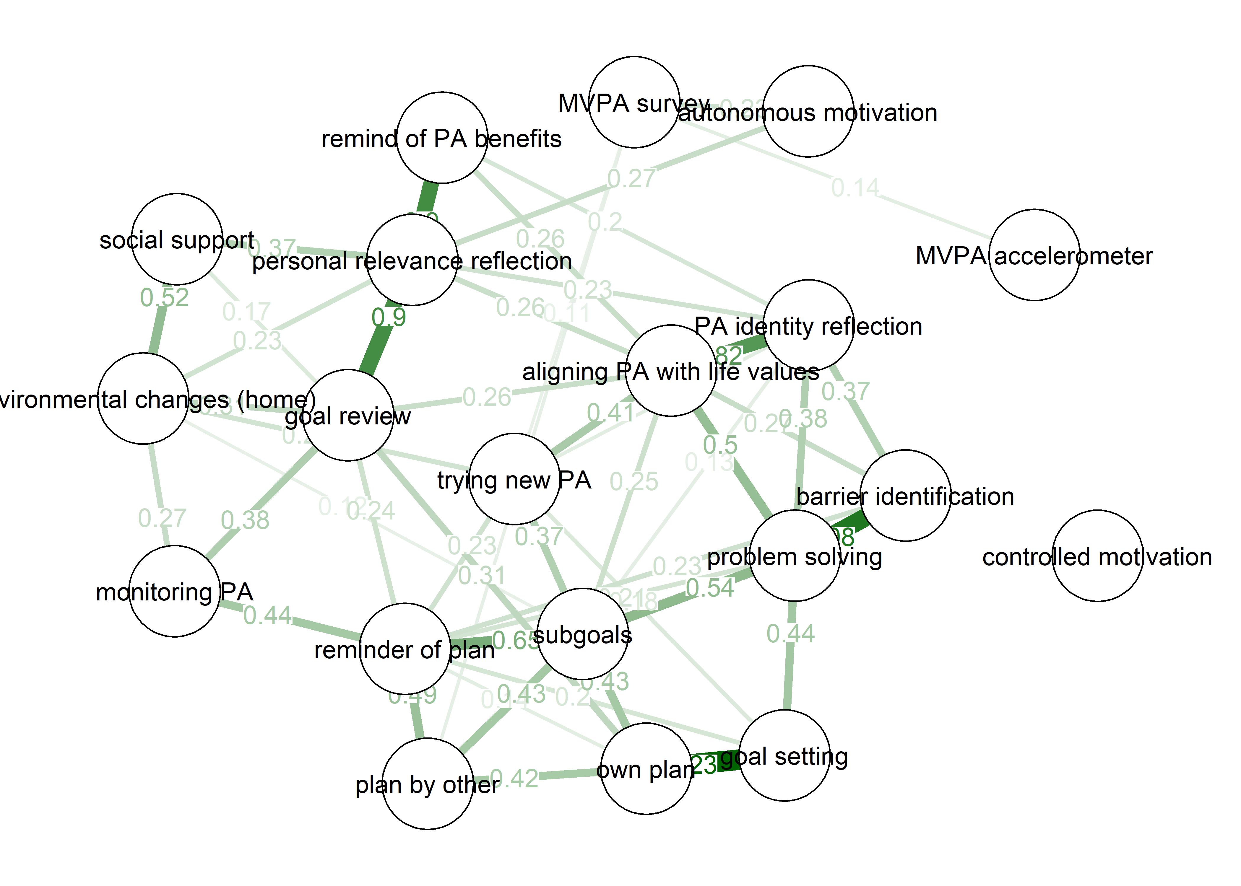
Controlled motivation with nonparanormal transformation
The nonparanormal transformation can alleviate normality issues, and the controlled motivation variable was heavily skewed. In our case, though, applying the non-paranormal transformation introduces a huge spike in the distribution, as it is not a skewed normal (results, not shown, introduced a positive edge between social support and controlled motivation). As the distribution resembles poisson, we treat controlled motivation variable as poisson below. Results do not change.
bctdf_mgm_T1 <- df %>% dplyr::select(
#  id,
#  intervention,
#  group,
#  school,
#  girl,
  'goal setting' = PA_agreementDependentBCT_01_T1,
  'own plan' = PA_agreementDependentBCT_02_T1,
  'plan by other' = PA_agreementDependentBCT_03_T1,
  'reminder of plan' = PA_agreementDependentBCT_04_T1,
  'subgoals' = PA_agreementDependentBCT_05_T1,
  'trying new PA' = PA_agreementDependentBCT_06_T1,
  'barrier identification' = PA_agreementDependentBCT_07_T1,
  'problem solving' = PA_agreementDependentBCT_08_T1,
  'PA identity reflection' = PA_agreementDependentBCT_09_T1,
  'aligning PA with life values' = PA_agreementDependentBCT_10_T1,
  'remind of PA benefits' = PA_frequencyDependentBCT_01_T1,
  'self-monitor (paper)' = PA_frequencyDependentBCT_02_T1,
  'self-monitor (app)' = PA_frequencyDependentBCT_03_T1,
#  'memory cues' = PA_frequencyDependentBCT_04_T1, # Issues with clarity of item wording
  'goal review' = PA_frequencyDependentBCT_05_T1,
  'personal relevance reflection' = PA_frequencyDependentBCT_06_T1,
  'environmental changes (home)' = PA_frequencyDependentBCT_07_T1,
  'social support' = PA_frequencyDependentBCT_08_T1,
  'analysing goal failure' = PA_frequencyDependentBCT_09_T1,
  'MVPA survey' = padaysLastweek_T1,
  'MVPA accelerometer' = mvpaAccelerometer_T1,
  'intrinsic' = PA_intrinsic_T1,
  'identified' = PA_identified_T1, 'integrated' = PA_integrated_T1,
  PA_controlled_01_T1, PA_controlled_02_T1, PA_controlled_03_T1, PA_controlled_04_T1, PA_controlled_05_T1) %>%
 rowwise() %>%
 mutate(
  'goal setting' = ifelse(`goal setting` == 1, 0, 1),
#  'has plan' = ifelse(`own plan` == 1 & `plan by other` == 1, 0, 1),
  'own plan' = ifelse(`own plan` == 1, 0, 1),
  'plan by other' = ifelse(`plan by other` == 1, 0, 1),
  'reminder of plan' = ifelse(`reminder of plan` == 1, 0, 1),
  'subgoals' = ifelse(`subgoals` == 1, 0, 1),
  'trying new PA' = ifelse(`trying new PA` == 1, 0, 1),
  'barrier identification' = ifelse(`barrier identification` == 1, 0, 1),
  'problem solving' = ifelse(`problem solving` == 1, 0, 1),
  # 'barriers identified or planned for' = ifelse(`problem solving` == 1 & `barrier identification` == 1, 0, 1),
  'PA identity reflection' = ifelse(`PA identity reflection` == 1, 0, 1),
  'aligning PA with life values' = ifelse(`aligning PA with life values` == 1, 0, 1),
  # 'identity, life values' = ifelse(`PA identity reflection` == 1 & `aligning PA with life values` == 1, 0, 1),
  'remind of PA benefits' = ifelse(`remind of PA benefits` == 1, 0, 1),
  'monitoring PA' = ifelse(`self-monitor (paper)` == 1 & `self-monitor (app)` == 1, 0, 1),
#  'memory cues' = ifelse(`memory cues` == 1, 0, 1),
  'goal review' = ifelse(`goal review` == 1, 0, 1),
  'personal relevance reflection' = ifelse(`personal relevance reflection` == 1, 0, 1),
  'environmental changes (home)' = ifelse(`environmental changes (home)` == 1, 0, 1),
  'social support' = ifelse(`social support` == 1, 0, 1),
  'analysing goal failure' = ifelse(`analysing goal failure` == 1, 0, 1),
  'autonomous motivation' = mean(c(identified, intrinsic, integrated), na.rm = T),
#  'girl' = ifelse(girl == "girl", 1, 0),
  'controlled motivation' = PA_controlled_01_T1 + PA_controlled_02_T1 + PA_controlled_03_T1 + PA_controlled_04_T1 + PA_controlled_05_T1) %>%  # If "at least partly" or more true + input 1. Normality otherwise a problem.
#  'intervention' = ifelse(intervention == "1", 1, 0)) %>%
  dplyr::select(-`self-monitor (paper)`, -`self-monitor (app)`,
                # -`plan by other`, -`own plan`,
                -identified, -intrinsic, -integrated,
                -PA_controlled_01_T1, -PA_controlled_02_T1, -PA_controlled_03_T1,
                -PA_controlled_04_T1, -PA_controlled_05_T1,
         -`analysing goal failure` # only concerns those who haven't reached goals
         # -`barrier identification`, -`problem solving`, # closely related
           ) %>%
#  dplyr::select(-controlled) %>% # Not really gaussian at all
  dplyr::select('MVPA survey', 'MVPA accelerometer', everything())

# # Non-paranormal transformation introduces a huge spike in the distribution, as it is not a skewed normal.
# bctdf_mgm_T1$`controlled motivation` <- huge::huge.npn(bctdf_mgm_T1$`controlled motivation` %>% data.matrix)
bctdf_mgm_T1$`autonomous motivation`[is.nan(bctdf_mgm_T1$`autonomous motivation`)] <- NA

labs <- names(bctdf_mgm_T1)

# mgm wants full data, see package missForest for imputation methods
bctdf_mgm_T1 <- bctdf_mgm_T1 %>% na.omit(.)
# bctdf_mgm %>% names()
mgm_variable_types <- c("g", "g", rep("c", 16), "g", "p")
mgm_variable_levels <- c("1", "1", rep("2", 16), "1", "1")
# data.frame(mgm_variable_types, mgm_variable_levels, names(bctdf_mgm))

mgm_obj_T1 <- mgm::mgm(data = bctdf_mgm_T1,
  type = mgm_variable_types,
  level = mgm_variable_levels,
  lambdaSel = "EBIC",
  # lambdaFolds = 10,
  verbatim = FALSE,
  pbar = FALSE,
  binarySign = TRUE)
## Note that the sign of parameter estimates is stored separately; see ?mgm

# Node pies:
pies_T1 <- bctdf_mgm_T1 %>%
  colMeans() # results in a series of means, which is ok for dichotomous vars
pies_T1["MVPA survey"] <- pies_T1["MVPA survey"] / 7
pies_T1["MVPA accelerometer"] <- pies_T1["MVPA accelerometer"] / max(bctdf_mgm_T1$`MVPA accelerometer`, na.rm = TRUE)
pies_T1["autonomous motivation"] <- pies_T1["autonomous motivation"] / 5
pies_T1["controlled motivation"] <- pies_T1["controlled motivation"] / max(bctdf_mgm_T1$`controlled motivation`, na.rm = TRUE)

node_colors <- c(viridis::viridis(3, begin = 0.4, end = 0.99)[1], # Color 1 for MVPA (questionnaire)
                 viridis::viridis(3, begin = 0.4, end = 0.99)[1], # Color 1 for MVPA (accelerometer)
                 rep(viridis::viridis(3, begin = 0.4, end = 0.99)[2], 15), # 11x Color 2 for BCTs
                 rep(viridis::viridis(3, begin = 0.4, end = 0.99)[3], 1), # Color 3 for motivation (controlled)
                 rep(viridis::viridis(3, begin = 0.4, end = 0.99)[2], 1), # 1x Color 2 for BCTs
                 viridis::viridis(3, begin = 0.4, end = 0.99)[3]) # Color 3 for motivation (autonomous)

BCT_mgm_T1 <- qgraph::qgraph(mgm_obj_T1$pairwise$wadj,
            layout = "spring",
            repulsion = 0.99, # To nudge the network from originally bad visual state
            edge.color = ifelse(mgm_obj_T1$pairwise$edgecolor == "darkgreen", "blue", mgm_obj_T1$pairwise$edgecolor),
            pie = pies_T1,
            # pieColor = pie_colors_T1,
            pieColor = node_colors,
            labels = names(bctdf_mgm_T1),
            pieBorder = 1,
            label.cex = 0.75,
            cut = 0,
            edge.labels = TRUE,
            label.scale = FALSE,
            DoNotPlot = TRUE)

plot(BCT_mgm_T1)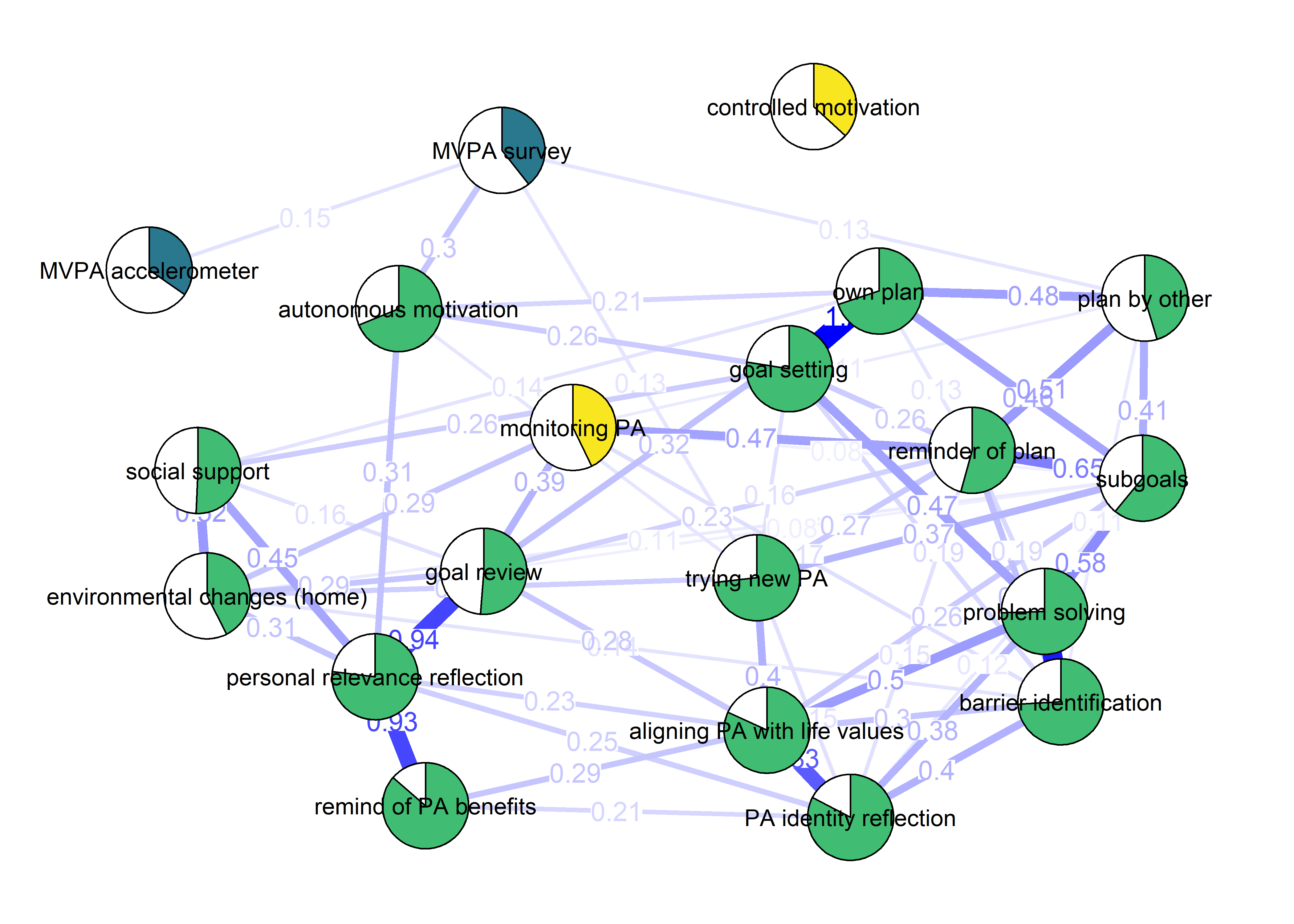
BCT_mgm_T1_circle <- qgraph::qgraph(mgm_obj_T1$pairwise$wadj,
            layout = "circle",
            title = "Mixed graphical model: PA, BCTs & motivation",
            edge.color = ifelse(mgm_obj_T1$pairwise$edgecolor == "darkgreen", "blue", mgm_obj_T1$pairwise$edgecolor),
            pie = pies_T1,
            pieColor = viridis::viridis(5, begin = 0.3, end = 0.8)[5],
            color = node_colors,
            labels = names(bctdf_mgm_T1),
            label.cex = 0.75,
            cut = 0,
            label.scale = FALSE,
            DoNotPlot = TRUE)

plot(BCT_mgm_T1_circle)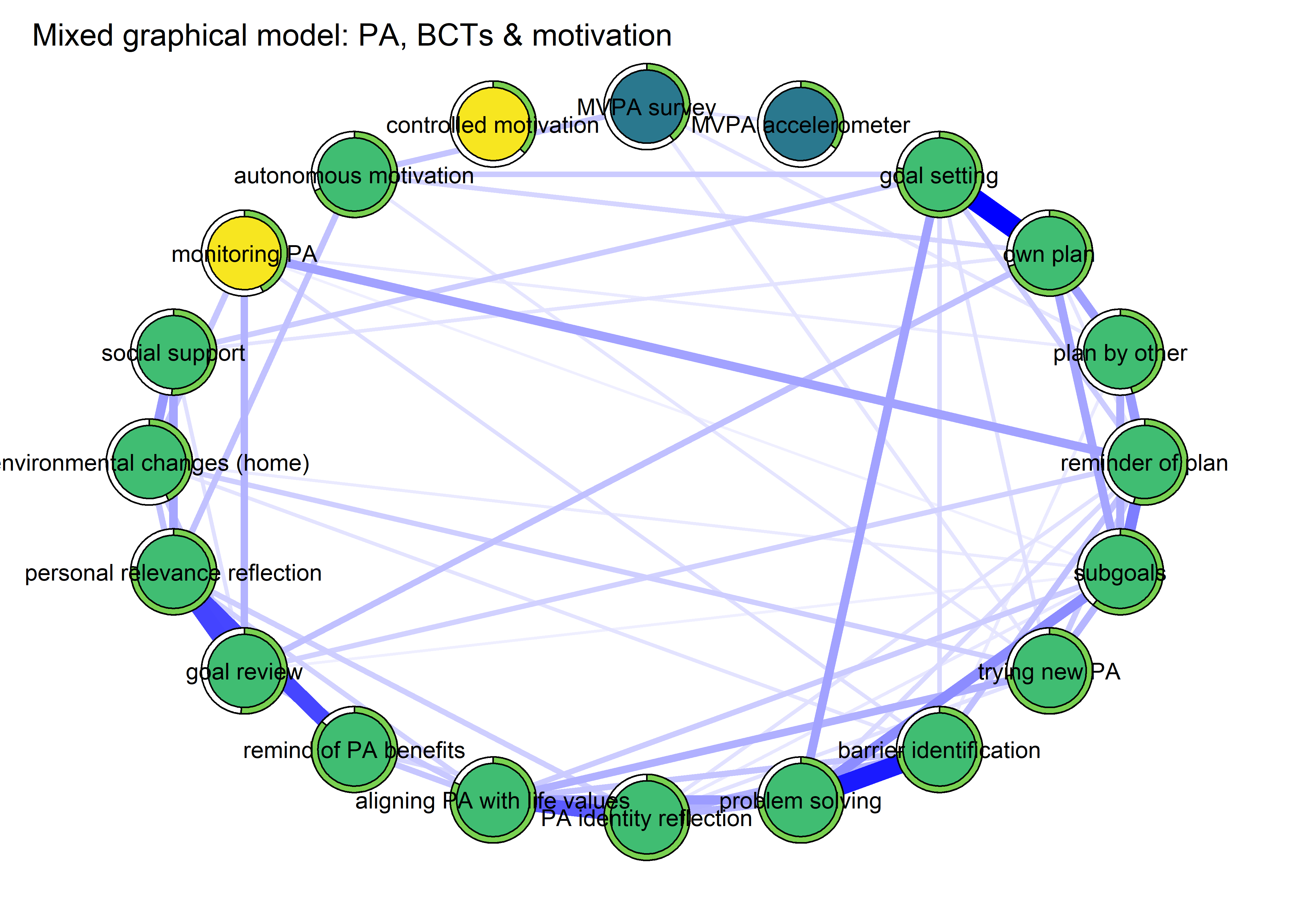
Combined BCT chunks
The following network depicts a mixed graphical model, with the following variables:
Two measures of physical activity.
MVPA accelerometeris the mean accelerometer-measured Moderate-to-Vigorous Physical Activity (MVPA) during a day in the measurement period,MVPA questionnaireis a survey item which asked “on how many days the previous week were you active for at least 30 minutes so, that you were out of breath”.One Behaviour Change Technique usage node (BCT usage is the mean of all techniques participants reported having used).
Four motivation types (Intrinsic and Identified, which are facets of “autonomous regulation” according to the self-determination theory, looked normal so used as continuous. Introjected and Extrinsic - facets of “controlled regulation” - were heavily skewed, so they were dichotomised: if “at least partly” or more true, a participant gets 1, otherwise 0.
bctdf_mgm <- df %>% dplyr::select(
  'agr-BCTs' = PA_agreementDependentBCT_T1,
  'frq-BCTs' = PA_frequencyDependentBCT_T1,
  'MVPA questionnaire' = padaysLastweek_T1,
  'MVPA accelerometer' = mvpaAccelerometer_T1,
  'Intrinsic' = PA_intrinsic_T1,
  'Identified' = PA_identified_T1,
  'Introjected' = PA_introjected_T1,
  'Extrinsic' = PA_extrinsic_T1) %>%
 rowwise() %>%
 mutate(
  'BCT usage' = mean(c(`agr-BCTs`, `frq-BCTs`), na.rm = TRUE),
  # 'autonomous motivation' = mean(c(identified, intrinsic), na.rm = TRUE),
  'Extrinsic' = ifelse(`Extrinsic` < 3, 0, 1), # If "at least partly" or more true, input 1. Normality otherwise a problem.
  'Introjected' = ifelse(`Introjected` < 3, 0, 1)) %>%  # If "at least partly" or more true, input 1. Normality otherwise a problem.
  dplyr::select('MVPA questionnaire', 'MVPA accelerometer', 'BCT usage', everything(), -contains("-BCTs")) %>%
  mutate_all(as.numeric)

bctdf_mgm$`BCT usage`[is.nan(bctdf_mgm$`BCT usage`)] <- NA


# If you need mock data:
# bctdf_mgm <- data.frame(
#   'MVPA questionnaire' = sample(1:8, size = 700, replace = TRUE),
#   'MVPA accelerometer' = rnorm(mean = 130, sd = 40, n = 700),
#   'BCT usage' = replicate(19, sample(1:5, 700, rep = TRUE)) %>% as.data.frame() %>% rowMeans(.),
#   'Intrinsic' = replicate(3, sample(1:5, 700, rep = TRUE)) %>% as.data.frame() %>% rowMeans(.),
#   'Identified' = replicate(3, sample(1:5, 700, rep = TRUE)) %>% as.data.frame() %>% rowMeans(.),
#   'Introjected' = sample(0:1, 700, rep = TRUE) %>% as.data.frame() %>% rowMeans(.),
#   'Extrinsic' = sample(0:1, 700, rep = TRUE) %>% as.data.frame() %>% rowMeans(.)
# )

labs <- names(bctdf_mgm)

# mgm wants full data, see package missForest for imputation methods
bctdf_mgm <- bctdf_mgm %>% na.omit(.)
# bctdf_mgm %>% names()
mgm_variable_types <- c(rep("g", 5), "c", "c")
mgm_variable_levels <- c(rep("1", 5), "2", "2")
# data.frame(mgm_variable_types, mgm_variable_levels, names(bctdf_mgm))

mgm_obj <- mgm::mgm(data = bctdf_mgm,
  type = mgm_variable_types,
  level = mgm_variable_levels,
  lambdaSel = "CV",
  lambdaFolds = 10,
  pbar = FALSE,
  binarySign = TRUE)
## Note that the sign of parameter estimates is stored separately; see ?mgm

pred_obj <- predict(object = mgm_obj,
                         data = bctdf_mgm)

pred_obj$errors
# Take R2 from gaussian, CC from categorical variables
pie_errors <- c(pred_obj$errors[1:5, 3],
                pred_obj$errors[6:7, 4])

# Coloring nodes: make a sequence of colors from the viridis palette. We need three colors (MVPA, BCTs, motivation), and "begin" from ones that are not too dark, so that black text shows up ok.

node_colors <- c(viridis::viridis(5, begin = 0.4, end = 0.99)[1], # Color 1 for MVPA (questionnaire)
                 viridis::viridis(5, begin = 0.4, end = 0.99)[1], # Color 1 for MVPA (accelerometer)
                 rep(viridis::viridis(5, begin = 0.4, end = 0.99)[4], 1), # 1x Color 4 for BCTs
                 rep(viridis::viridis(5, begin = 0.4, end = 0.99)[2], 2), # 2x Color 2 for autonomous
                 rep(viridis::viridis(5, begin = 0.4, end = 0.99)[3], 2)) # 2x Color 3 for controlled

BCT_mgm <- qgraph::qgraph(mgm_obj$pairwise$wadj,
            layout = "spring",
            repulsion = 1, # To nudge the network from originally bad visual state
            # title = "Mixed graphical model: PA, BCTs & motivation",
            edge.color = ifelse(mgm_obj$pairwise$edgecolor == "darkgreen", "blue", mgm_obj$pairwise$edgecolor),
            pie = pie_errors,
            pieColor = viridis::viridis(5, begin = 0.3, end = 0.8)[5],
            color = node_colors,
            labels = names(bctdf_mgm),
            label.cex = 0.8,
            label.scale = FALSE,
            node.width = 1.65)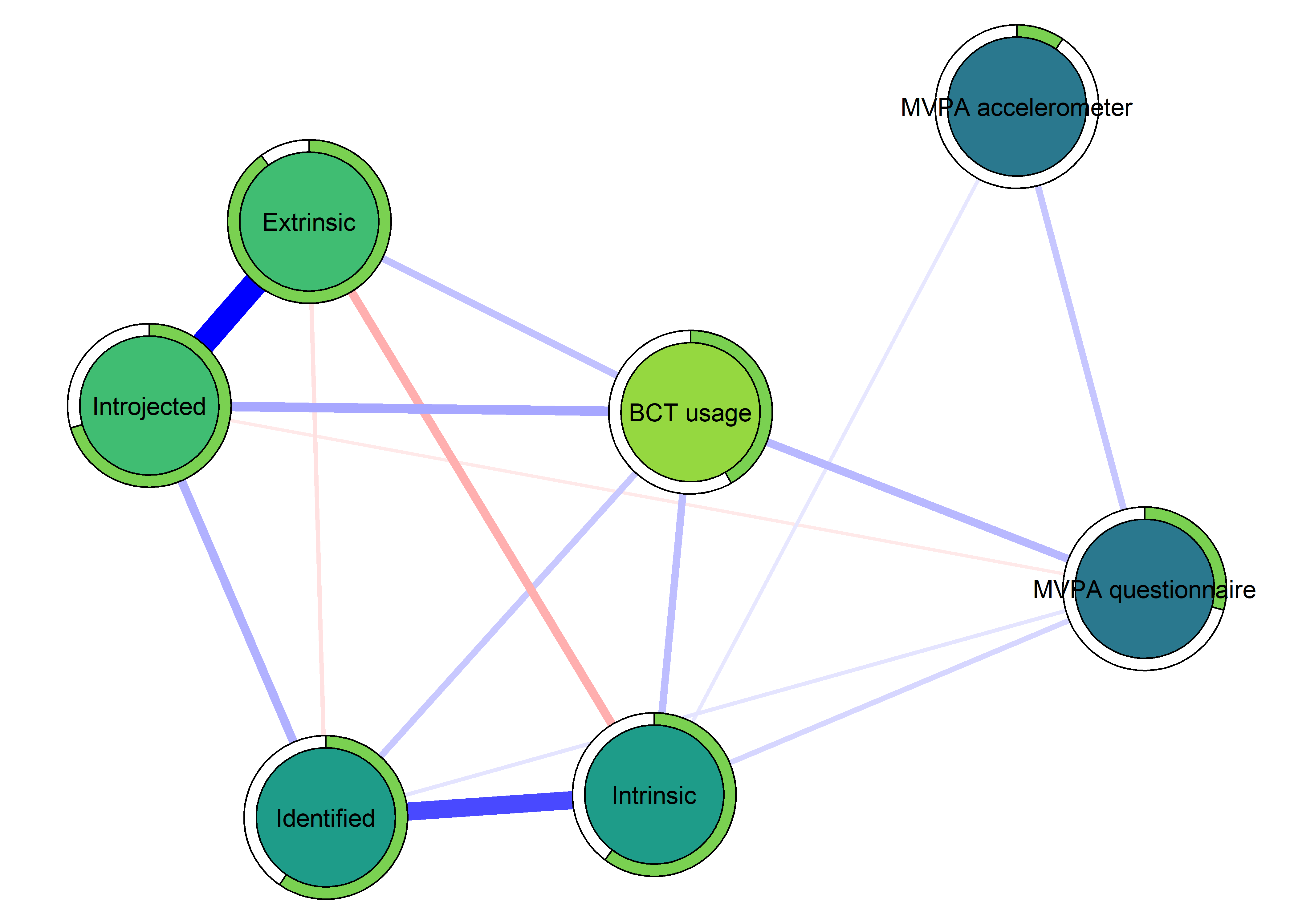
adjacency_noAmotivation <- mgm_obj$pairwise$wadj
save(adjacency_noAmotivation, file = "./Rdata_files/adjacency_noAmotivation.Rdata")
signs_noAmotivation <- mgm_obj$pairwise$signs
save(signs_noAmotivation, file = "./Rdata_files/signs_noAmotivation.Rdata")
# BCT_mgm_noAmotivation_stability <- mgm::resample(object = mgm_obj, data = bctdf_mgm, nB = 100)
# save(BCT_mgm_noAmotivation_stability, file = "./Rdata_files/BCT_mgm_noAmotivation_stability.Rdata")
load("./Rdata_files/BCT_mgm_noAmotivation_stability.Rdata")

# # Plotting the bootstrapped edge between variables 1 and 4:
# hist(BCT_mgm_noAmotivation_stability$bootParameters[1, 4, ],
# main = "",
# xlab = "Parameter Estimate")

mgm::plotRes(object = BCT_mgm_noAmotivation_stability,
        quantiles = c(.05, .95),
        cex.label = 0.5,
        lwd.qtl = 2.5,
        cex.mean = .5,
        labels = names(bctdf_mgm))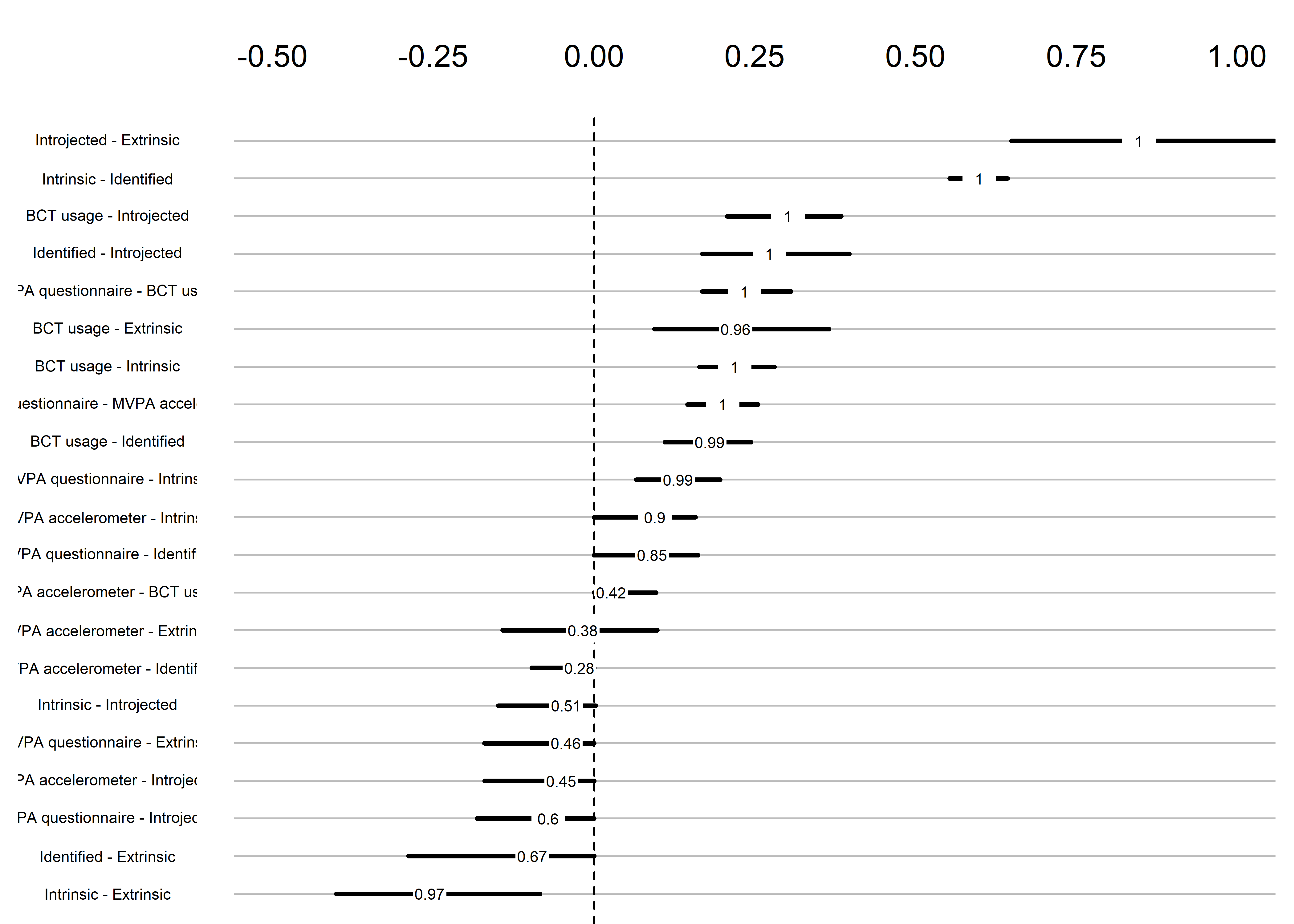
The bootstrap stability plot above shows the proportion of re-samples, which contain a non-zero link between two edges (for a tutorial, see this link – or, if it’s down, this archived page). For example, when we draw observations from the current sample with replacement a 100 times, 99% of these times a non-zero link between questionnaire-measured MVPA and intrinsic motivation is estimated.
Correlation network and mixed graphical model compared
## Note that the sign of parameter estimates is stored separately; see ?mgm
averagedLayout <- qgraph::averageLayout(BCT_mgm, corgraph)

layout(t(1:2))

BCT_mgm <- qgraph::qgraph(mgm_obj$pairwise$wadj,
            layout = averagedLayout,
            edge.color = ifelse(mgm_obj$pairwise$edgecolor == "darkgreen", "blue", mgm_obj$pairwise$edgecolor),
            pie = pie_errors,
            pieColor = viridis::viridis(5, begin = 0.3, end = 0.99)[2],
            color = node_colors,
            labels = names(bctdf_mgm),
            # label.cex = 1,
            label.scale = FALSE,
            # node.width = 1,
            edge.labels = TRUE,
            title = "A)")

corgraph <- qgraph::qgraph(qgraph::cor_auto(bctdf_mgm),
              layout = averagedLayout,
              graph = "cor",
              pie = piefill,
              pieBorder = 1,
              pieColor = node_colors,
              labels = names(bctdf_mgm),
              # label.cex = 1,
              label.scale = FALSE,
              # node.width = 1,
              edge.labels = TRUE,
              title = "B)")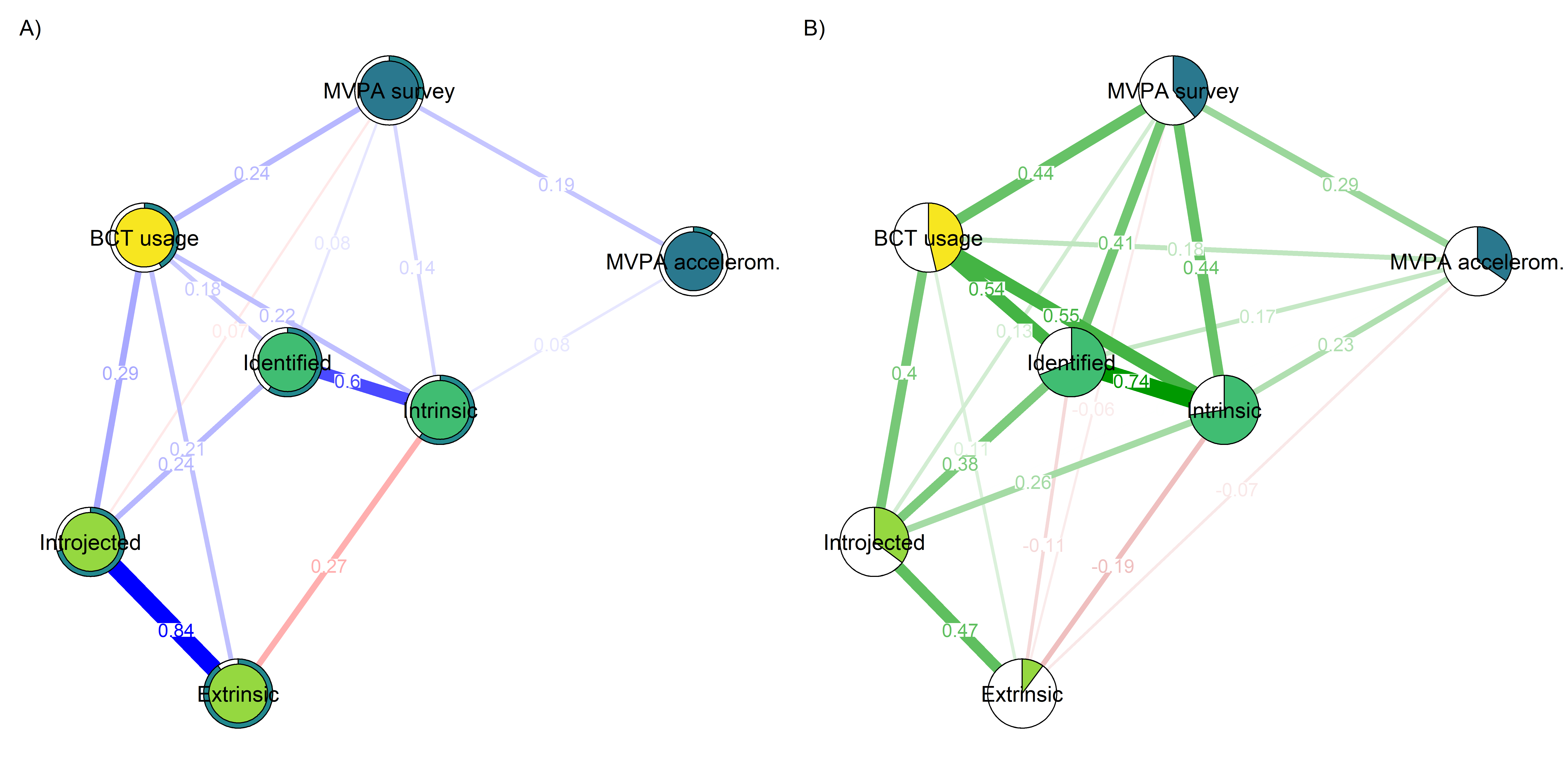
- Mixed graphical model with LASSO regularisation and model selection by cross-validation. Pie indicates node predictability. B) Bivariate correlation network. Pie indicates node mean as % of theoretical maximum (for MVPA accelerometer, mean as % maximum observed MVPA).
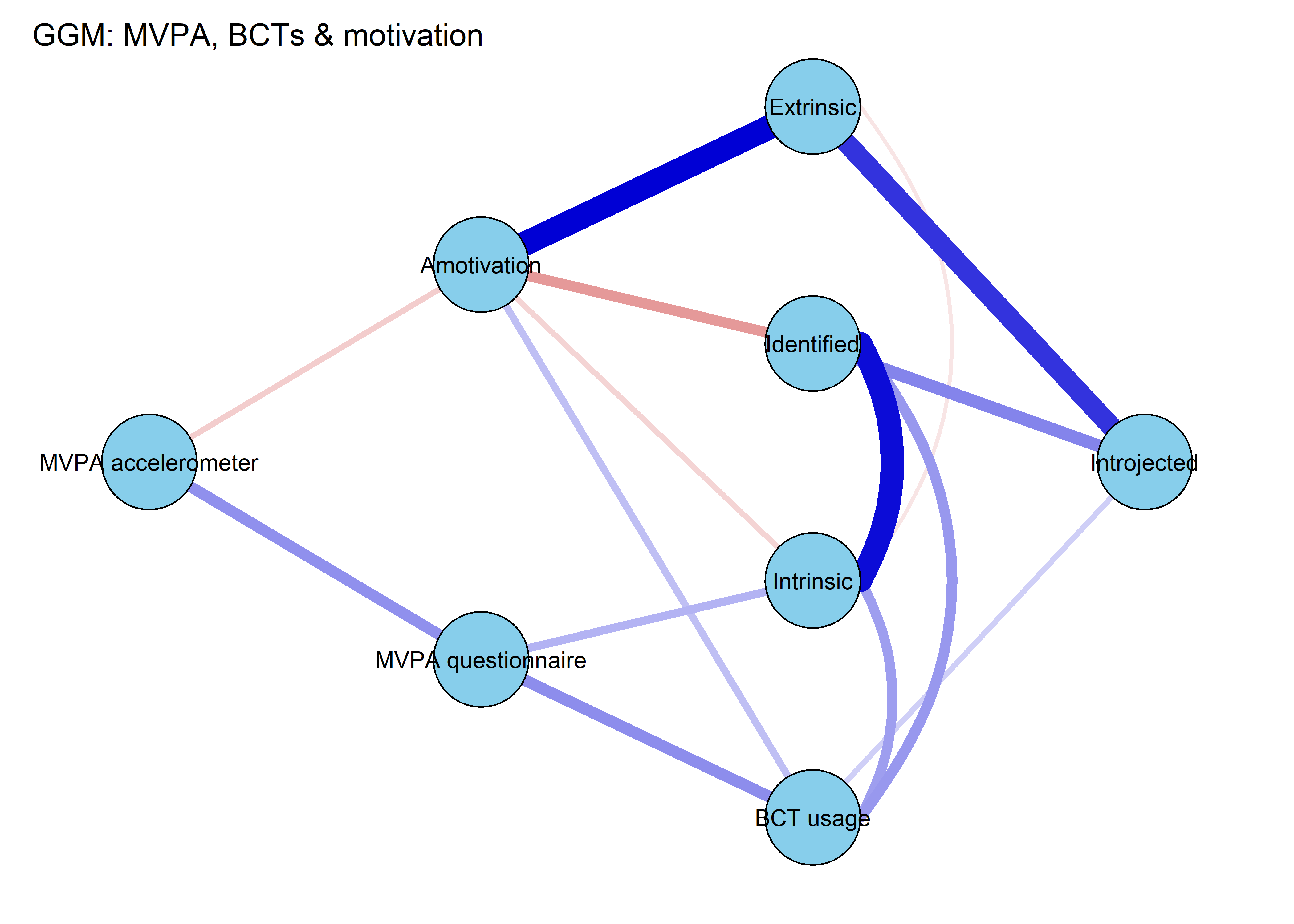
The “last motivation type”, i.e. the fifth, is Amotivation (dichotomised due to skew). A node for that is added in the network below:
bctdf_mgm <- df %>% dplyr::select(
  'agr-BCTs' = PA_agreementDependentBCT_T1,
  'frq-BCTs' = PA_frequencyDependentBCT_T1,
  'MVPA questionnaire' = padaysLastweek_T1,
  'MVPA accelerometer' = mvpaAccelerometer_T1,
  'Intrinsic' = PA_intrinsic_T1,
  'Identified' = PA_identified_T1,
  'Introjected' = PA_introjected_T1,
  'Extrinsic' = PA_extrinsic_T1,
  'Amotivation' = PA_amotivation_T1) %>%
 rowwise() %>%
 mutate(
  'BCT usage' = mean(c(`agr-BCTs`, `frq-BCTs`), na.rm = TRUE),
  # 'autonomous motivation' = mean(c(identified, intrinsic), na.rm = TRUE),
  'Extrinsic' = ifelse(`Extrinsic` < 3, 0, 1), # If "at least partly" or more true, input 1. Normality otherwise a problem.
  'Amotivation' = ifelse(`Amotivation` < 3, 0, 1), # If "at least partly" or more true, input 1. Normality otherwise a problem.
  'Introjected' = ifelse(`Introjected` < 3, 0, 1)) %>%  # If "at least partly" or more true, input 1. Normality otherwise a problem.
  dplyr::select('MVPA questionnaire', 'MVPA accelerometer', 'BCT usage', everything(), -contains("-BCTs")) %>%
  mutate_all(as.numeric)

bctdf_mgm$`BCT usage`[is.nan(bctdf_mgm$`BCT usage`)] <- NA

labs <- names(bctdf_mgm)

# mgm wants full data, see package missForest for imputation methods
bctdf_mgm <- bctdf_mgm %>% na.omit(.)
# bctdf_mgm %>% names()
mgm_variable_types <- c(rep("g", 5), "c", "c", "c")
mgm_variable_levels <- c(rep("1", 5), "2", "2", "2")
# data.frame(mgm_variable_types, mgm_variable_levels, names(bctdf_mgm))

mgm_obj <- mgm::mgm(data = bctdf_mgm,
  type = mgm_variable_types,
  level = mgm_variable_levels,
  lambdaSel = "CV",
  lambdaFolds = 10,
  pbar = FALSE,
  binarySign = TRUE)
## Note that the sign of parameter estimates is stored separately; see ?mgm

pred_obj <- predict(object = mgm_obj,
                         data = bctdf_mgm)

pred_obj$errors
# Take R2 from gaussian, CC from categorical variables
pie_errors <- c(pred_obj$errors[1:5, 3],
                pred_obj$errors[6:8, 4])

# Coloring nodes: make a sequence of colors from the viridis palette. We need three colors (MVPA, BCTs, motivation), and "begin" from ones that are not too dark, so that black text shows up ok.

node_colors <- c(viridis::viridis(5, begin = 0.4, end = 0.99)[1], # Color 1 for MVPA (questionnaire)
                 viridis::viridis(5, begin = 0.4, end = 0.99)[1], # Color 1 for MVPA (accelerometer)
                 rep(viridis::viridis(5, begin = 0.4, end = 0.99)[4], 1), # 1x Color 4 for BCTs
                 rep(viridis::viridis(5, begin = 0.4, end = 0.99)[2], 2), # 2x Color 2 for autonomous
                 rep(viridis::viridis(5, begin = 0.4, end = 0.99)[3], 3)) # 3x Color 3 for controlled/amotivation

BCT_mgm <- qgraph::qgraph(mgm_obj$pairwise$wadj,
            layout = "spring",
            repulsion = 1, # To nudge the network from originally bad visual state
            # title = "Mixed graphical model: PA, BCTs & motivation",
            edge.color = ifelse(mgm_obj$pairwise$edgecolor == "darkgreen", "blue", mgm_obj$pairwise$edgecolor),
            pie = pie_errors,
            pieColor = viridis::viridis(5, begin = 0.3, end = 0.8)[5],
            color = node_colors,
            labels = names(bctdf_mgm),
            label.cex = 0.8,
            label.scale = FALSE,
            node.width = 1.65)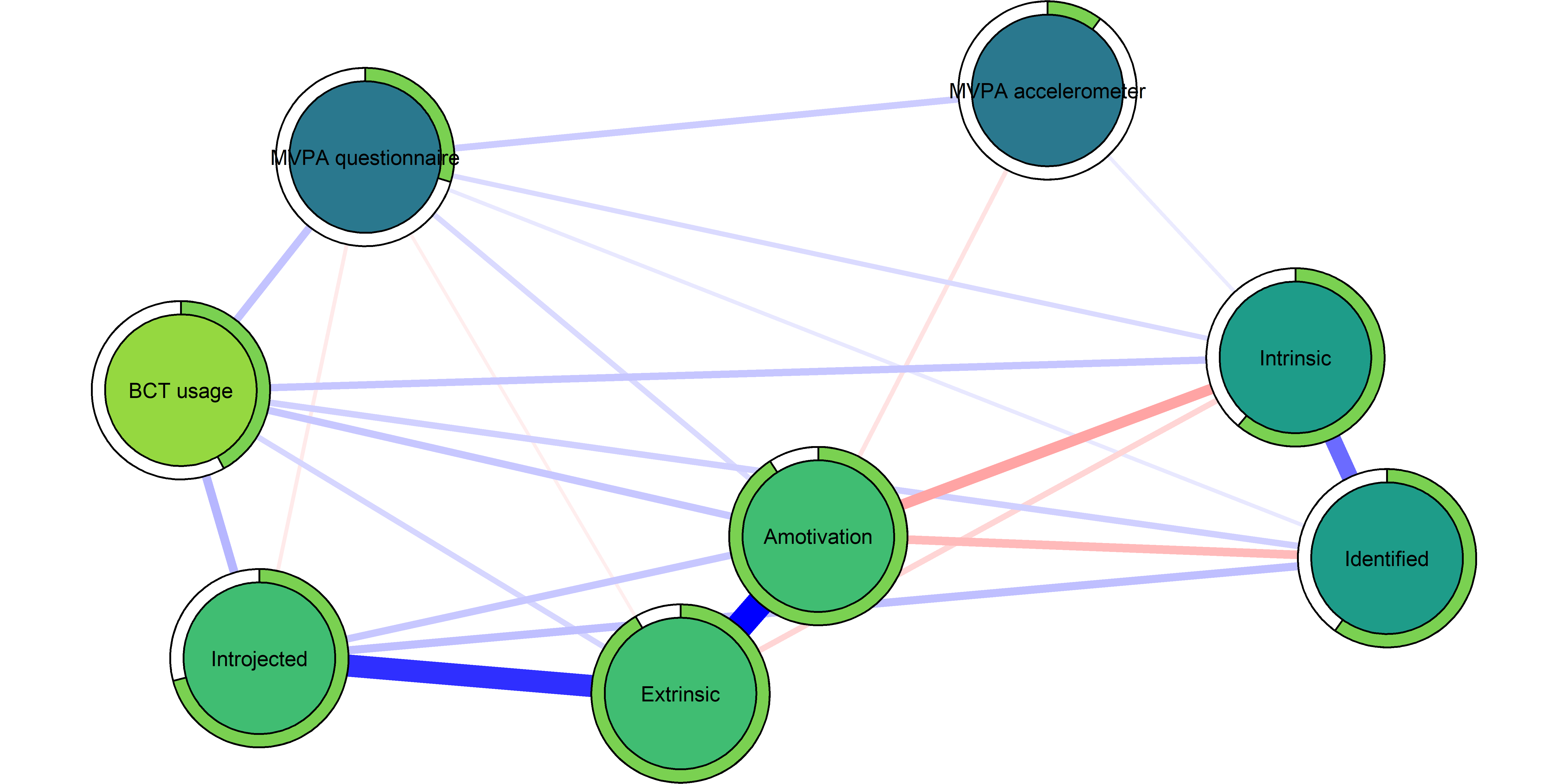
# BCT_mgm_withAmotivation_stability <- mgm::resample(object = mgm_obj, data = bctdf_mgm, nB = 100)
# save(BCT_mgm_withAmotivation_stability, file = "./Rdata_files/BCT_mgm_withAmotivation_stability.Rdata")
load("./Rdata_files/BCT_mgm_withAmotivation_stability.Rdata")

mgm::plotRes(object = BCT_mgm_withAmotivation_stability,
        quantiles = c(.05, .95),
        cex.label = 0.5,
        lwd.qtl = 2.5,
        labels = bctdf_mgm %>% names(),
        cex.mean = .5)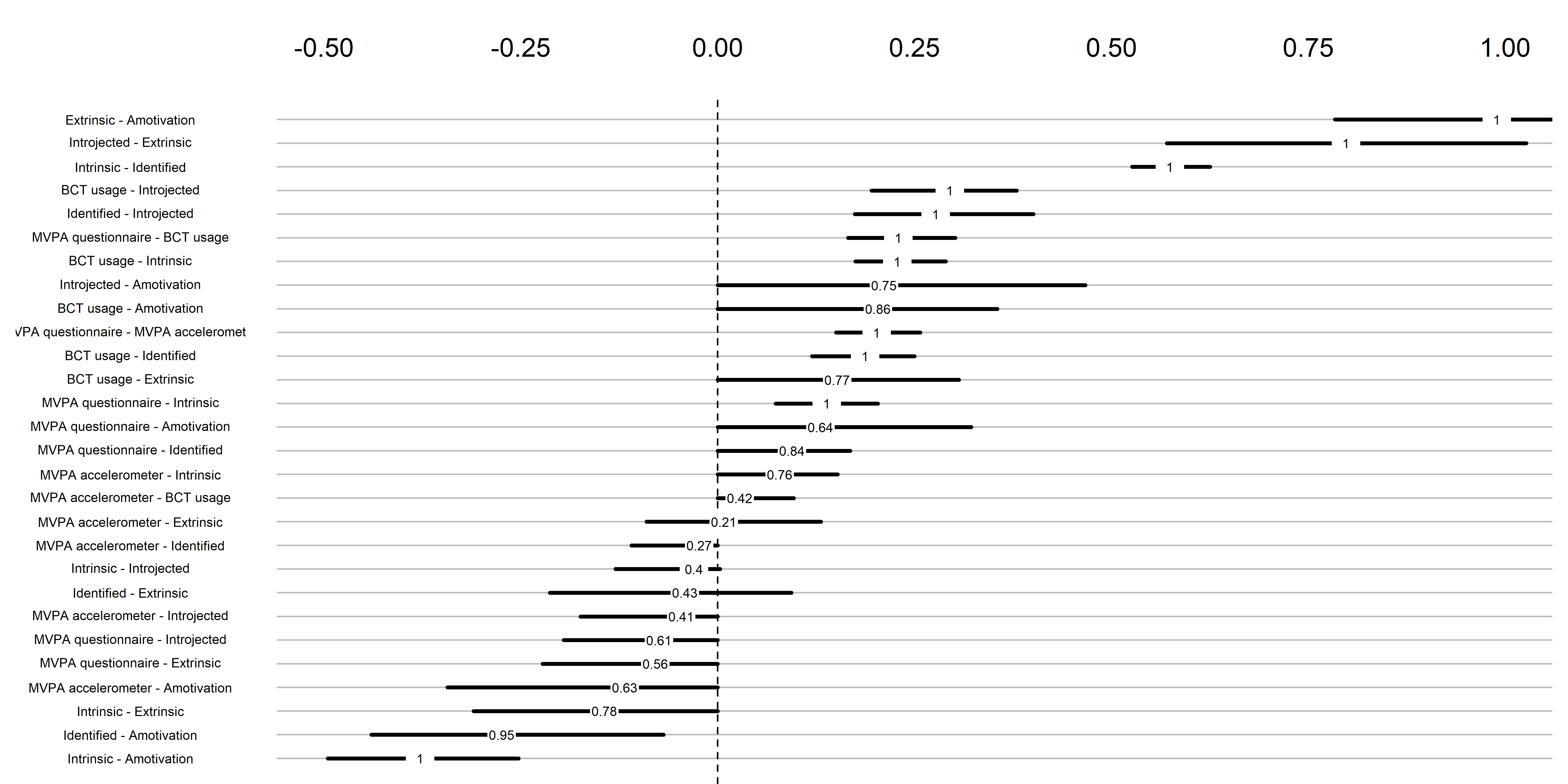
Theory-wise, Amotivation should be negatively correlated with everything but Extrinsic and Introjected. Given that BCT usage is 19 items, there are probably a lot of ways there can be a positive correlation, although that would be unexpected. But the positive relation with MVPA questionnaire would mean, that people who report having done physical activity on more days last week, would also say they don’t see any point in doing physical activity (another example item: I think exercising is a waste of time). One explanation would be some form of conditioning on a collider.
One option would be, that (as the model drops incomplete observations), there is some selection effects based on motivation types and/or BCT usage. To check for this, we estimate a Gaussian Graphical Model, which assumes normally distributed data but uses all observations.
bctdf_ggm <- df %>% dplyr::select(
  'agr-BCTs' = PA_agreementDependentBCT_T1,
  'frq-BCTs' = PA_frequencyDependentBCT_T1,
  'MVPA questionnaire' = padaysLastweek_T1,
  'MVPA accelerometer' = mvpaAccelerometer_T1,
  'Intrinsic' = PA_intrinsic_T1,
  'Identified' = PA_identified_T1,
  'Introjected' = PA_introjected_T1,
  'Extrinsic' = PA_extrinsic_T1,
  'Amotivation' = PA_amotivation_T1) %>%
 rowwise() %>%
 mutate(
  'BCT usage' = mean(c(`agr-BCTs`, `frq-BCTs`), na.rm = TRUE),
  # 'autonomous motivation' = mean(c(identified, intrinsic), na.rm = TRUE),
  'Extrinsic' = ifelse(`Extrinsic` < 3, 0, 1), # If "at least partly" or more true, input 1. Normality otherwise a problem.
  'Amotivation' = ifelse(`Amotivation` < 3, 0, 1), # If "at least partly" or more true, input 1. Normality otherwise a problem.
  'Introjected' = ifelse(`Introjected` < 3, 0, 1)) %>%  # If "at least partly" or more true, input 1. Normality otherwise a problem.
  dplyr::select('MVPA questionnaire', 'MVPA accelerometer', 'BCT usage', everything(), -contains("-BCTs")) %>%
  mutate_all(as.numeric)

bctdf_ggm$`BCT usage`[is.nan(bctdf_ggm$`BCT usage`)] <- NA

# Network for all participants
S.total_ggm <- bctdf_ggm
nwBCT_ggm <- bootnet::estimateNetwork(S.total_ggm, default="ggmModSelect")

labs_ggm <- colnames(S.total_ggm)

# Create means for filling nodes
# piefill_ggm <- S.total_ggm %>%
#   dplyr::select(-contains("MVPA"), -contains("motivation")) %>% data.frame %>%
#   dplyr::summarise_all(funs(mean(., na.rm = TRUE) /6))
#
# piefill_ggm$`MVPA accelerometer` <- median(S.total_ggm$`MVPA accelerometer`, na.rm = TRUE) / (60 * 24)
# piefill_ggm$`MVPA questionnaire` <- median(S.total_ggm$`MVPA questionnaire`, na.rm = TRUE) / 7
# piefill_ggm$autonomous <- median(S.total_ggm$`autonomous motivation`, na.rm = TRUE) / 5
# piefill_ggm$controlled <- median(S.total_ggm$`controlled motivation`, na.rm = TRUE) / 5
#
# piefill_ggm <- piefill_ggm %>%
#   dplyr::select("MVPA questionnaire", "MVPA accelerometer", autonomous, controlled, everything())

# Plot network

BCT_ggm <- plot(nwBCT_ggm,
                layout = "spring",
                repulsion = 0.99, # To nudge the network from originally bad visual state
                label.scale = FALSE,
                title = "GGM: MVPA, BCTs & motivation",
                label.cex = 0.75,
                # pie = piefill_ggm,
                color = "skyblue",
                pieBorder = 1)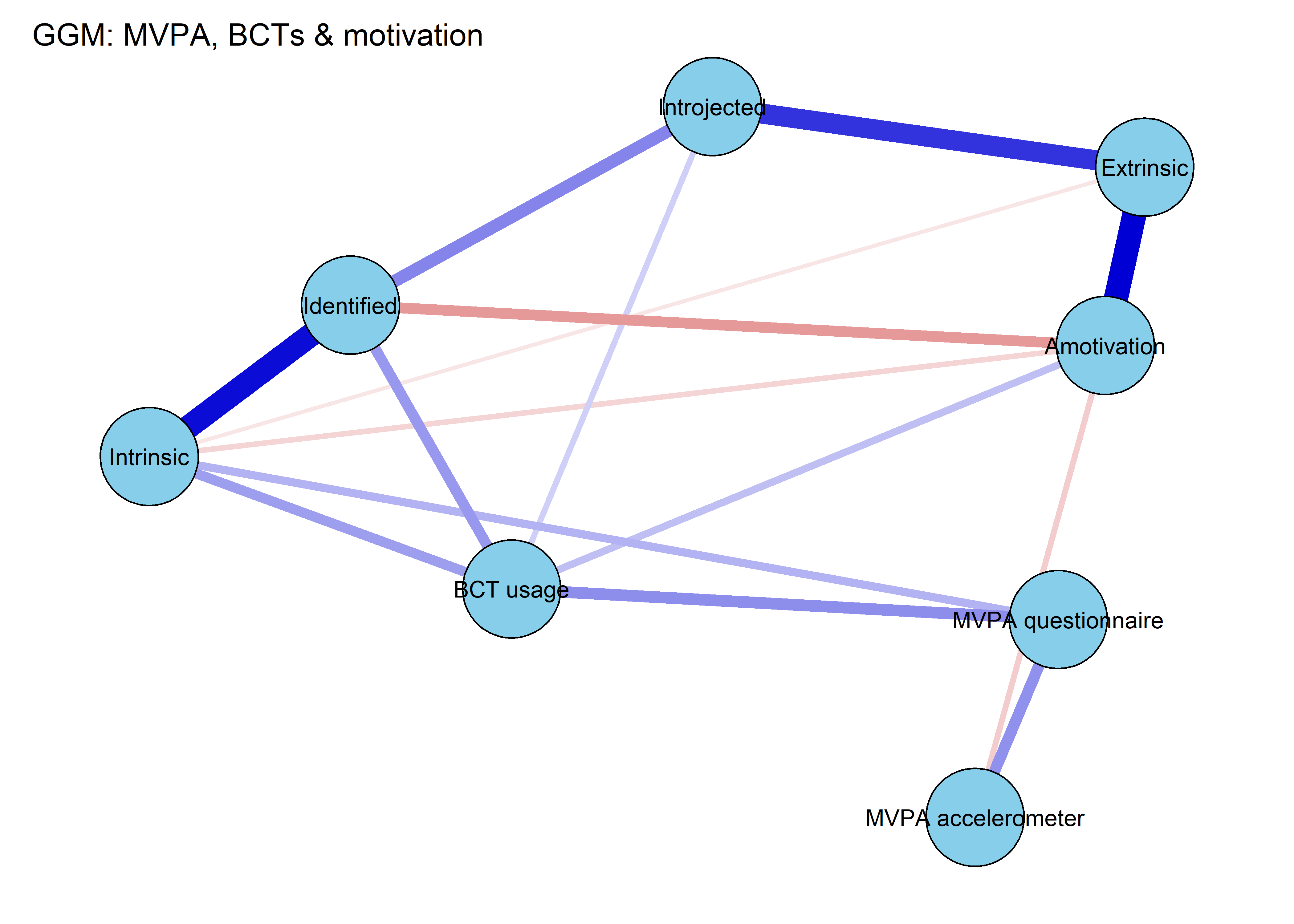
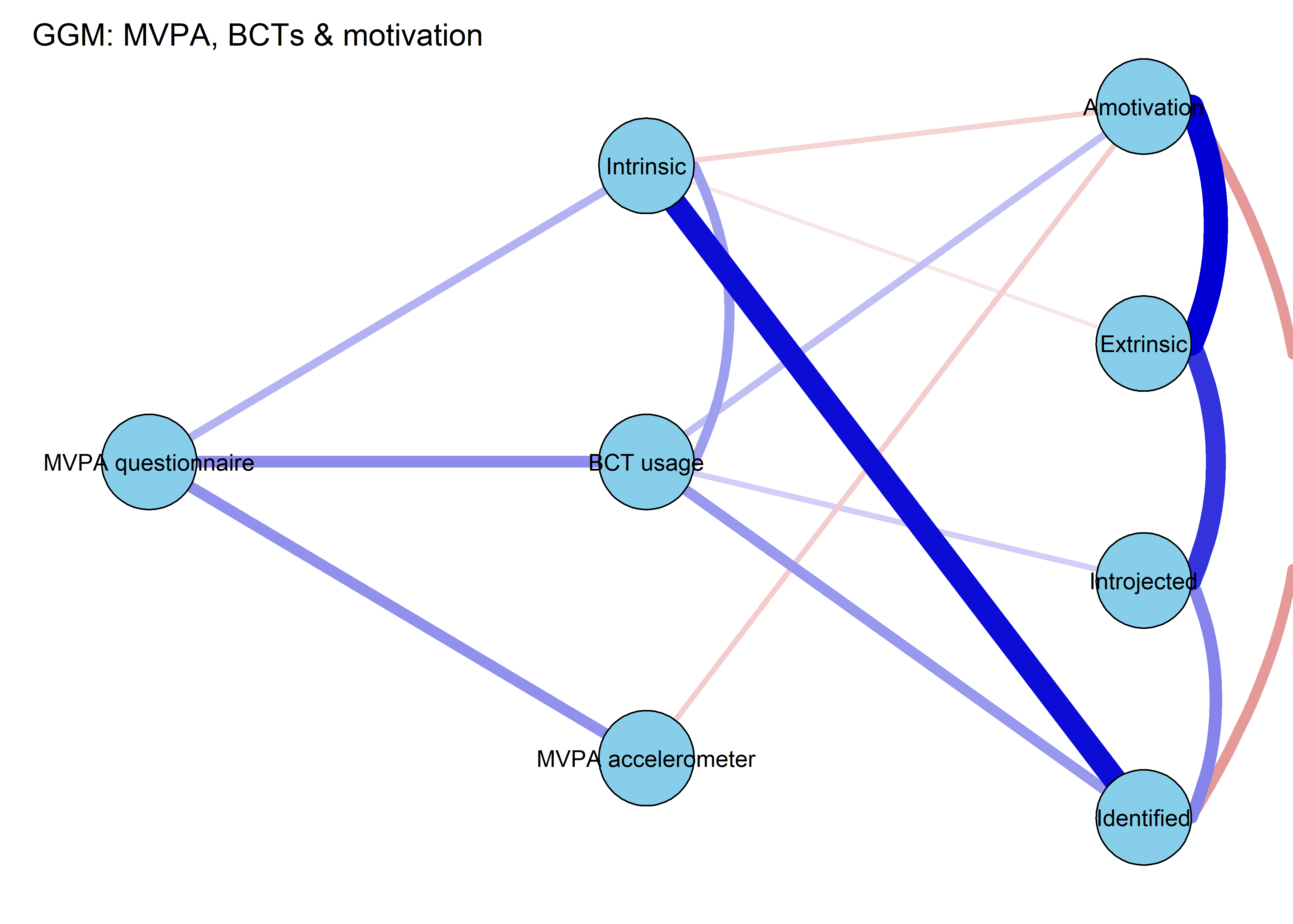
From the network above, we see that the positive connection between amotivation and questionnaire-measured MVPA has almost completely disappered. Bootstrapping to inspect stability shows, that the connection is likely to be zero (see 13th edge from the bottom; “MVPA questionnaire–Amotivation”).
# collider_boot <- bootnet(nwBCT_ggm, nBoots = 2500)
# save(collider_boot, file = "./Rdata_files/collider_boot.Rdata")
load("./Rdata_files/collider_boot.Rdata")
plot(collider_boot, plot = "interval", split0 = TRUE, order = "sample", labels = TRUE)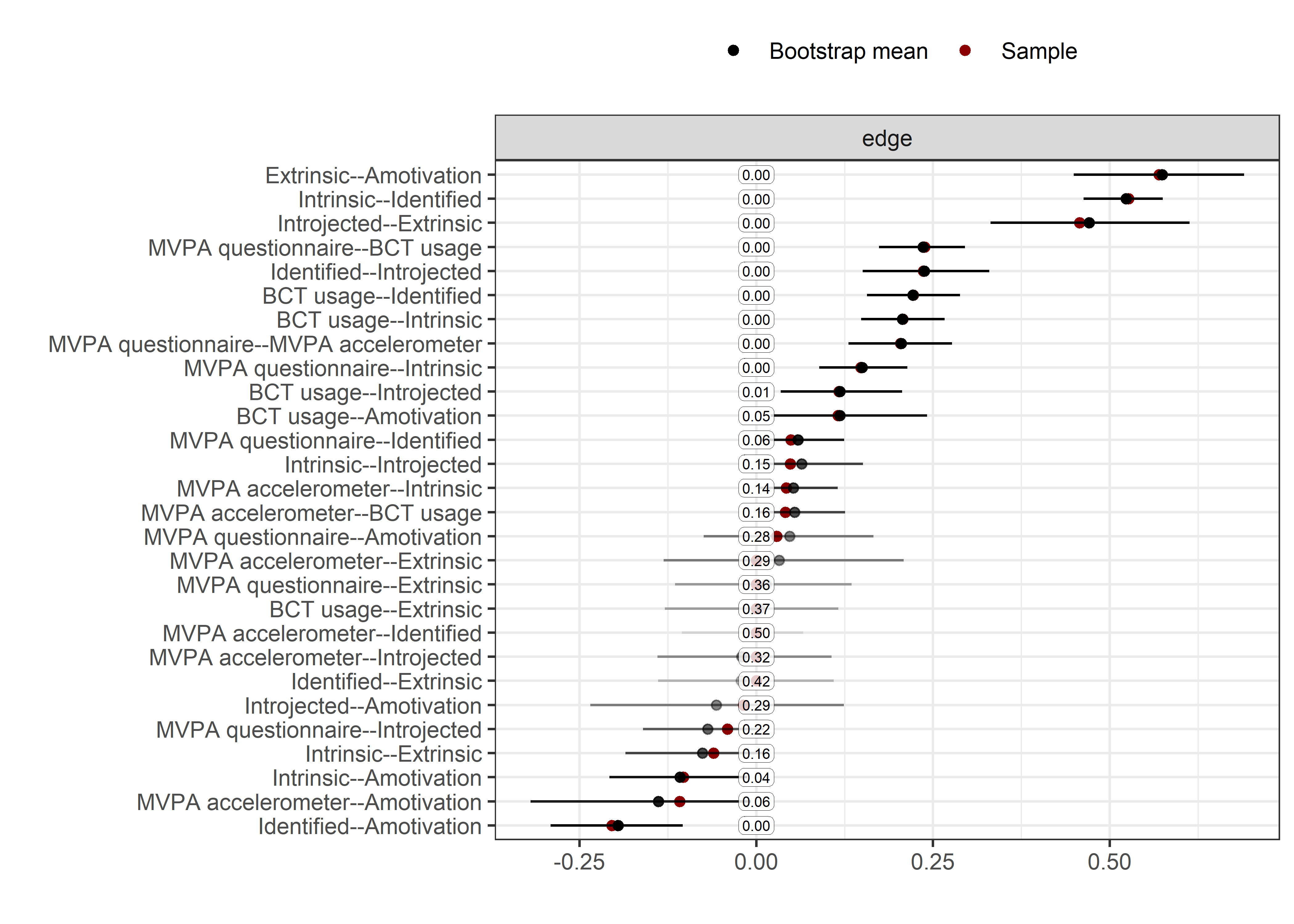
The bootstrap stability plot above (for a tutorial, see this link – or, if it’s down, this archived page) shows, that when we draw observations from the sample with replacement 2500 times, the connection between amotivation and questionnaire-measured MVPA was estimated as non-zero only about 30% of time.
Combining some BCT items
This section presents a Mixed Graphical Model (MGM) and a Gaussian Graphical Model (GGM). In the MGM, we opted to dichotomise the BCTs in order to increase interpretability while not violating model assumptions. Results do not differ very much. Some nodes were still combined, to reduce estimation burden.
bctdf_mgm <- df %>% dplyr::select(
#  id,
#  intervention,
#  group,
#  school,
#  girl,
  'goal setting' = PA_agreementDependentBCT_01_T1,
  'own plan' = PA_agreementDependentBCT_02_T1,
  'plan by other' = PA_agreementDependentBCT_03_T1,
  'reminder of plan' = PA_agreementDependentBCT_04_T1,
  'subgoals' = PA_agreementDependentBCT_05_T1,
  'trying new PA' = PA_agreementDependentBCT_06_T1,
  'barrier identification' = PA_agreementDependentBCT_07_T1,
  'problem solving' = PA_agreementDependentBCT_08_T1,
  'PA identity reflection' = PA_agreementDependentBCT_09_T1,
  'aligning PA with life values' = PA_agreementDependentBCT_10_T1,
  'remind of PA benefits' = PA_frequencyDependentBCT_01_T1,
  'self-monitor (paper)' = PA_frequencyDependentBCT_02_T1,
  'self-monitor (app)' = PA_frequencyDependentBCT_03_T1,
#  'memory cues' = PA_frequencyDependentBCT_04_T1, # Issues with clarity of item wording
  'goal review' = PA_frequencyDependentBCT_05_T1,
  'personal relevance reflection' = PA_frequencyDependentBCT_06_T1,
  'environmental changes (home)' = PA_frequencyDependentBCT_07_T1,
  'social support' = PA_frequencyDependentBCT_08_T1,
  'analysing goal failure' = PA_frequencyDependentBCT_09_T1,
  'MVPA questionnaire' = padaysLastweek_T1,
  'MVPA accelerometer' = mvpaAccelerometer_T1,
  'intrinsic' = PA_intrinsic_T1,
  'identified' = PA_identified_T1,
  'controlled motivation' = PA_controlled_T1) %>%
 rowwise() %>%
 mutate(
  'goal setting' = ifelse(`goal setting` == 1, 0, 1),
#  'has plan' = ifelse(`own plan` == 1 & `plan by other` == 1, 0, 1),
  'own plan' = ifelse(`own plan` == 1, 0, 1),
  'plan by other' = ifelse(`plan by other` == 1, 0, 1),
  'reminder of plan' = ifelse(`reminder of plan` == 1, 0, 1),
  'subgoals' = ifelse(`subgoals` == 1, 0, 1),
  'trying new PA' = ifelse(`trying new PA` == 1, 0, 1),
#  'barrier identification' = ifelse(`barrier identification` == 1, 0, 1),
#  'problem solving' = ifelse(`problem solving` == 1, 0, 1),
  'barriers identified or planned for' = ifelse(`problem solving` == 1 & `barrier identification` == 1, 0, 1),
#  'PA identity reflection' = ifelse(`PA identity reflection` == 1, 0, 1),
#  'aligning PA with life values' = ifelse(`aligning PA with life values` == 1, 0, 1),
  'identity, life values' = ifelse(`PA identity reflection` == 1 & `aligning PA with life values` == 1, 0, 1),
  'remind of PA benefits' = ifelse(`remind of PA benefits` == 1, 0, 1),
  'monitoring PA' = ifelse(`self-monitor (paper)` == 1 & `self-monitor (app)` == 1, 0, 1),
#  'memory cues' = ifelse(`memory cues` == 1, 0, 1),
  'goal review' = ifelse(`goal review` == 1, 0, 1),
  'personal relevance reflection' = ifelse(`personal relevance reflection` == 1, 0, 1),
  'environmental changes (home)' = ifelse(`environmental changes (home)` == 1, 0, 1),
  'social support' = ifelse(`social support` == 1, 0, 1),
  'analysing goal failure' = ifelse(`analysing goal failure` == 1, 0, 1),
  'autonomous motivation' = mean(c(identified, intrinsic), na.rm = T),
#  'girl' = ifelse(girl == "girl", 1, 0),
  'controlled motivation' = ifelse(`controlled motivation` < 3, 0, 1)) %>%  # If "at least partly" or more true, input 1. Normality otherwise a problem.
#  'intervention' = ifelse(intervention == "1", 1, 0)) %>%
  dplyr::select(-`self-monitor (paper)`, -`self-monitor (app)`,
                # -`plan by other`, -`own plan`,
                -identified, -intrinsic,
         -`analysing goal failure`, # only concerns those who haven't reached goals
         -`barrier identification`, -`problem solving`, # closely related
         -`PA identity reflection`, -`aligning PA with life values`) %>% # closely related
#  dplyr::select(-controlled) %>% # Not really gaussian at all
  dplyr::select('MVPA questionnaire', 'MVPA accelerometer', everything())

bctdf_mgm$`autonomous motivation`[is.nan(bctdf_mgm$`autonomous motivation`)] <- NA

labs <- names(bctdf_mgm)
mgm estimation
# devtools::install_github("jmbh/mgm")
# Restart R for the latest package
# .r.restartR()

# mgm wants full data, see package missForest for imputation methods
bctdf_mgm <- bctdf_mgm %>% na.omit(.)
# bctdf_mgm %>% names()
mgm_variable_types <- c("g", "g", rep("c", 15), "g")
mgm_variable_levels <- c("1", "1", rep("2", 15), "1")
# data.frame(mgm_variable_types, mgm_variable_levels, names(bctdf_mgm))

mgm_obj <- mgm::mgm(data = bctdf_mgm,
  type = mgm_variable_types,
  level = mgm_variable_levels,
  lambdaSel = "CV",
  lambdaFolds = 10,
  pbar = FALSE,
  binarySign = TRUE)
## Note that the sign of parameter estimates is stored separately; see ?mgm

pred_obj <- predict(object = mgm_obj,
                         data = bctdf_mgm)

pred_obj$errorsmgm plotting
# Coloring nodes: make a sequence of colors from the viridis palette. We need three colors (MVPA, BCTs, motivation), and "begin" from ones that are not too dark, so that black text shows up ok.

node_colors <- c(viridis::viridis(3, begin = 0.4, end = 0.99)[1], # Color 1 for MVPA (questionnaire)
                 viridis::viridis(3, begin = 0.4, end = 0.99)[1], # Color 1 for MVPA (accelerometer)
                 rep(viridis::viridis(3, begin = 0.4, end = 0.99)[2], 11), # 11x Color 2 for BCTs
                 rep(viridis::viridis(3, begin = 0.4, end = 0.99)[3], 1), # Color 3 for motivation (controlled)
                 rep(viridis::viridis(3, begin = 0.4, end = 0.99)[2], 3), # 3x Color 2 for BCTs
                 viridis::viridis(3, begin = 0.4, end = 0.99)[3]) # Color 3 for motivation (autonomous)

BCT_mgm <- qgraph::qgraph(mgm_obj$pairwise$wadj,
            layout = "spring",
            repulsion = 0.9999, # To nudge the network from originally bad visual state
            title = "Mixed graphical model: PA, BCTs & motivation",
            edge.color = ifelse(mgm_obj$pairwise$edgecolor == "darkgreen", "blue", mgm_obj$pairwise$edgecolor),
            pie = pie_errors,
            pieColor = viridis::viridis(5, begin = 0.3, end = 0.8)[5],
            color = node_colors,
            labels = names(bctdf_mgm),
            label.cex = 0.75,
            label.scale = FALSE)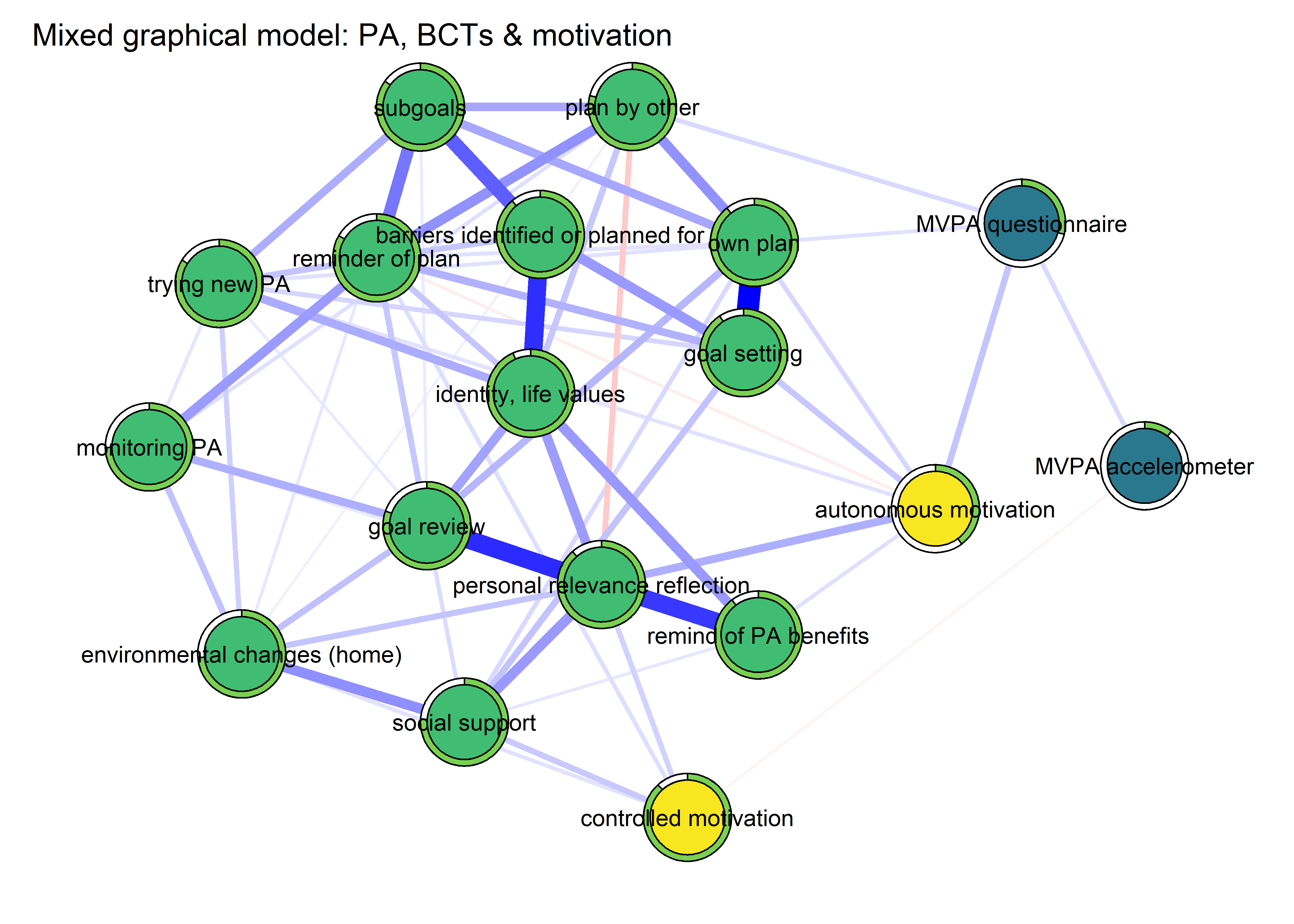
ggm estimation & plotting
bctdf_ggm <- df %>% dplyr::select(
#  id,
#  intervention,
#  group,
#  school,
#  girl,
  'goal setting' = PA_agreementDependentBCT_01_T1,
  'own plan' = PA_agreementDependentBCT_02_T1,
  'plan by other' = PA_agreementDependentBCT_03_T1,
  'reminder of plan' = PA_agreementDependentBCT_04_T1,
  'subgoals' = PA_agreementDependentBCT_05_T1,
  'trying new PA' = PA_agreementDependentBCT_06_T1,
  'barrier identification' = PA_agreementDependentBCT_07_T1,
  'problem solving' = PA_agreementDependentBCT_08_T1,
  'PA identity reflection' = PA_agreementDependentBCT_09_T1,
  'aligning PA with life values' = PA_agreementDependentBCT_10_T1,
  'remind of PA benefits' = PA_frequencyDependentBCT_01_T1,
  'self-monitor (paper)' = PA_frequencyDependentBCT_02_T1,
  'self-monitor (app)' = PA_frequencyDependentBCT_03_T1,
#  'memory cues' = PA_frequencyDependentBCT_04_T1,
  'goal review' = PA_frequencyDependentBCT_05_T1,
  'personal relevance reflection' = PA_frequencyDependentBCT_06_T1,
  'environmental changes (home)' = PA_frequencyDependentBCT_07_T1,
  'social support' = PA_frequencyDependentBCT_08_T1,
  'failure contemplated' = PA_frequencyDependentBCT_09_T1,
  'MVPA questionnaire' = padaysLastweek_T1,
  'MVPA accelerometer' = mvpaAccelerometer_T1,
  'intrinsic' = PA_intrinsic_T1,
  'identified' = PA_identified_T1,
  'controlled motivation' = PA_controlled_T1) %>%
 rowwise() %>%
 mutate(
#  'has plan' = mean(c(`own plan`, `plan by other`), na.rm = TRUE),
  'barriers identified or planned for' = mean(c(`problem solving`, `barrier identification`), na.rm = TRUE),
  'identity, life values' = mean(c(`PA identity reflection` == 1, `aligning PA with life values`), na.rm = TRUE),
  'monitoring PA' = mean(c(`self-monitor (paper)`, `self-monitor (app)`), na.rm = TRUE),
  'autonomous motivation' = mean(c(identified, intrinsic), na.rm = T)) %>%
#  'girl' = ifelse(girl == "girl", 1, 0),
#  'intervention' = ifelse(intervention == "1", 1, 0)) %>%
  dplyr::select(-`self-monitor (paper)`, -`self-monitor (app)`,
#                -`plan by other`, -`own plan`,
                -identified, -intrinsic,
         -`failure contemplated`, # only concerns those who haven't reached goals
         -`barrier identification`, -`problem solving`, # closely related
         -`PA identity reflection`, -`aligning PA with life values`) %>% # closely related
#  dplyr::select(-controlled) %>% # Not really gaussian at all
  dplyr::select("MVPA questionnaire", "MVPA accelerometer", "autonomous motivation", "controlled motivation", everything()) %>%
  dplyr::mutate_all(as.numeric)

# Network for all participants
S.total_ggm <- bctdf_ggm
nwBCT_ggm <- bootnet::estimateNetwork(S.total_ggm, default="ggmModSelect")

labs_ggm <- colnames(S.total_ggm)

# Create means for filling nodes
piefill_ggm <- S.total_ggm %>%
  dplyr::select(-contains("MVPA"), -contains("motivation")) %>% data.frame %>%
  dplyr::summarise_all(funs(mean(., na.rm = TRUE) /6))

piefill_ggm$`MVPA accelerometer` <- median(S.total_ggm$`MVPA accelerometer`, na.rm = TRUE) / (60 * 24)
piefill_ggm$`MVPA questionnaire` <- median(S.total_ggm$`MVPA questionnaire`, na.rm = TRUE) / 7
piefill_ggm$autonomous <- median(S.total_ggm$`autonomous motivation`, na.rm = TRUE) / 5
piefill_ggm$controlled <- median(S.total_ggm$`controlled motivation`, na.rm = TRUE) / 5

piefill_ggm <- piefill_ggm %>%
  dplyr::select("MVPA questionnaire", "MVPA accelerometer", autonomous, controlled, everything())

# Plot network

BCT_ggm <- plot(nwBCT_ggm,
                layout = "spring",
                repulsion = 0.99, # To nudge the network from originally bad visual state
                label.scale = FALSE,
                title = "GGM: MVPA, BCTs & motivation",
                label.cex = 0.75,
                pie = piefill_ggm,
                color = "skyblue",
                pieBorder = 1)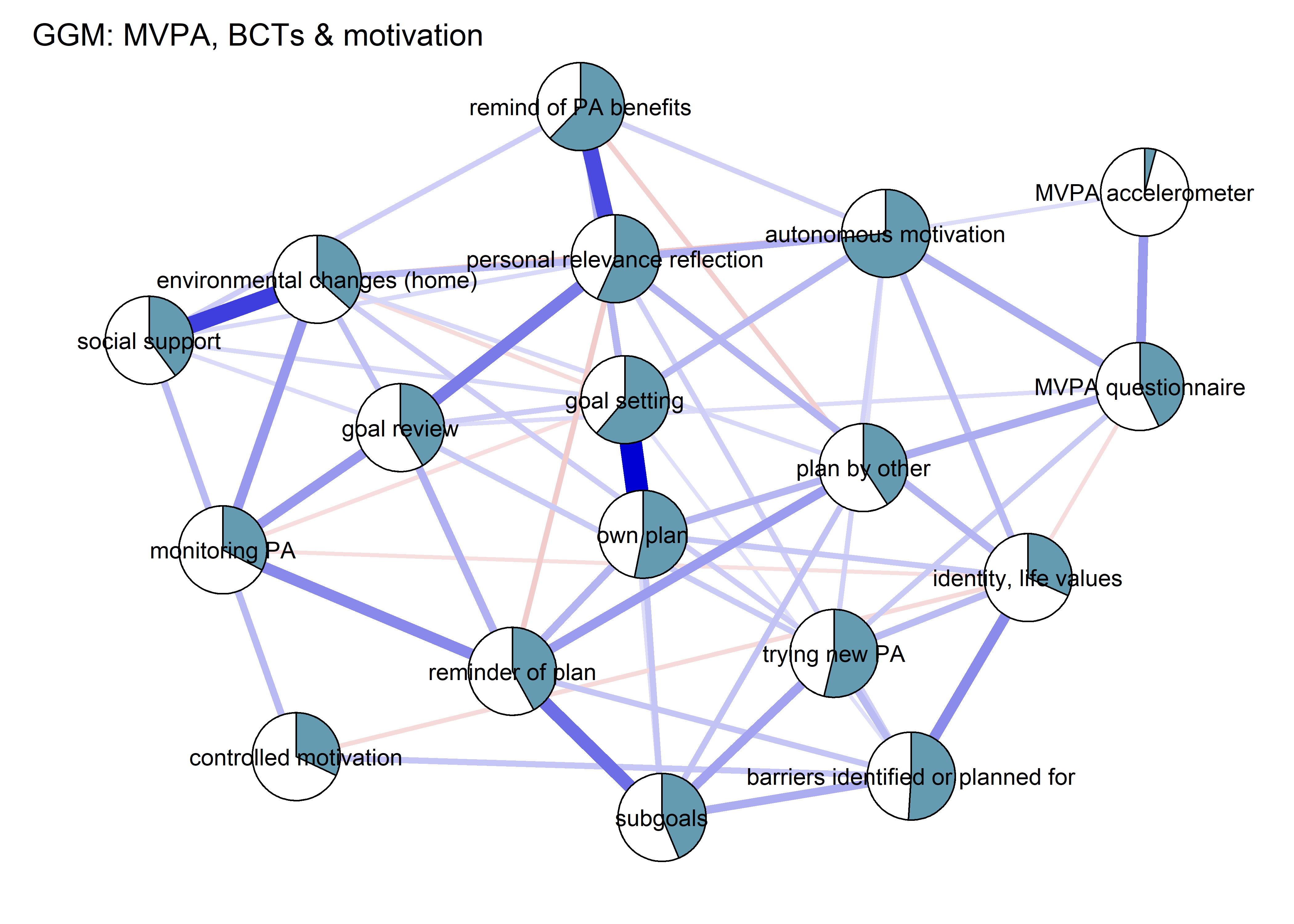
Centrality and stability
allBctsMotiSurveyPA <- nwBCT_ggm

allBctsMotiSurveyPA_centralityPlot <- qgraph::centralityPlot(allBctsMotiSurveyPA)
qgraph::centrality(allBctsMotiSurveyPA)$InDegree %>%
  data.frame("Node" = names(.), "Strength" = .) %>%
  dplyr::arrange(desc(Strength)) %>%
  papaja::apa_table()
## <caption>(\#tab:allBctsMotiSurveyPA-ggm-stability)</caption>
##
## <caption>**</caption>
##
##
##
## Node                                 Strength
## -----------------------------------  ---------
## personal relevance reflection        1.47
## reminder of plan                     1.37
## goal setting                         1.37
## environmental changes (home)         1.33
## goal review                          1.21
## autonomous motivation                1.13
## own plan                             1.13
## barriers identified or planned for   1.09
## subgoals                             1.04
## identity, life values                0.98
## plan by other                        0.96
## trying new PA                        0.94
## social support                       0.93
## remind of PA benefits                0.87
## MVPA questionnaire                   0.86
## monitoring PA                        0.85
## controlled motivation                0.36
## MVPA accelerometer                   0.30

scale(qgraph::centrality(allBctsMotiSurveyPA)$InDegree) %>%
  data.frame(Node = labels(.), `Standardised strength` = .) %>%
  plyr::arrange(desc(`Standardised.strength`)) %>%
  papaja::apa_table()
## <caption>(\#tab:allBctsMotiSurveyPA-ggm-stability)</caption>
##
## <caption>**</caption>
##
##
##
## Node.c..MVPA.questionnaire....MVPA.accelerometer....autonomous.motivation...   Node..1.   Standardised.strength
## -----------------------------------------------------------------------------  ---------  ----------------------
## personal relevance reflection                                                  1          1.48
## reminder of plan                                                               1          1.15
## goal setting                                                                   1          1.14
## environmental changes (home)                                                   1          1.02
## goal review                                                                    1          0.64
## autonomous motivation                                                          1          0.39
## own plan                                                                       1          0.37
## barriers identified or planned for                                             1          0.25
## subgoals                                                                       1          0.08
## identity, life values                                                          1          -0.08
## plan by other                                                                  1          -0.17
## trying new PA                                                                  1          -0.21
## social support                                                                 1          -0.25
## remind of PA benefits                                                          1          -0.45
## MVPA questionnaire                                                             1          -0.49
## monitoring PA                                                                  1          -0.51
## controlled motivation                                                          1          -2.08
## MVPA accelerometer                                                             1          -2.28

qgraph::centrality(allBctsMotiSurveyPA)$Closeness %>% data.frame(Closeness = .) %>% papaja::apa_table()
## <caption>(\#tab:allBctsMotiSurveyPA-ggm-stability)</caption>
##
## <caption>**</caption>
##
##
##
##                                      Closeness
## -----------------------------------  ----------
## MVPA questionnaire                   0.01
## MVPA accelerometer                   0.00
## autonomous motivation                0.01
## controlled motivation                0.00
## goal setting                         0.01
## own plan                             0.01
## plan by other                        0.01
## reminder of plan                     0.01
## subgoals                             0.01
## trying new PA                        0.01
## remind of PA benefits                0.01
## goal review                          0.01
## personal relevance reflection        0.01
## environmental changes (home)         0.01
## social support                       0.01
## barriers identified or planned for   0.01
## identity, life values                0.01
## monitoring PA                        0.01

qgraph::centrality(allBctsMotiSurveyPA)$Betweenness %>% data.frame(names(.), .) %>% papaja::apa_table()
## <caption>(\#tab:allBctsMotiSurveyPA-ggm-stability)</caption>
##
## <caption>**</caption>
##
##
##
##                                      names...                             .
## -----------------------------------  -----------------------------------  ------
## MVPA questionnaire                   MVPA questionnaire                   34.00
## MVPA accelerometer                   MVPA accelerometer                   0.00
## autonomous motivation                autonomous motivation                24.00
## controlled motivation                controlled motivation                2.00
## goal setting                         goal setting                         14.00
## own plan                             own plan                             18.00
## plan by other                        plan by other                        16.00
## reminder of plan                     reminder of plan                     32.00
## subgoals                             subgoals                             10.00
## trying new PA                        trying new PA                        4.00
## remind of PA benefits                remind of PA benefits                6.00
## goal review                          goal review                          10.00
## personal relevance reflection        personal relevance reflection        34.00
## environmental changes (home)         environmental changes (home)         34.00
## social support                       social support                       18.00
## barriers identified or planned for   barriers identified or planned for   16.00
## identity, life values                identity, life values                6.00
## monitoring PA                        monitoring PA                        10.00

cor(qgraph::centrality(allBctsMotiSurveyPA)$InDegree, qgraph::centrality(allBctsMotiSurveyPA)$Betweenness,
    method = "spearman")
## [1] 0.5978302

# bootnet_stability_allBctsMotiSurveyPA <- bootnet::bootnet(allBctsMotiSurveyPA, nBoots=1000)
# save(bootnet_stability_allBctsMotiSurveyPA, file = "./Rdata_files/bootnet_stability_allBctsMotiSurveyPA.Rdata")
load("./Rdata_files/bootnet_stability_allBctsMotiSurveyPA.Rdata")

plot(bootnet_stability_allBctsMotiSurveyPA, labels = FALSE, order = "sample") 
# bootnet_centrality_stability_allBctsMotiSurveyPA <- bootnet::bootnet(allBctsMotiSurveyPA, nBoots=1000,nCores=8, type="case")
# save(bootnet_centrality_stability_allBctsMotiSurveyPA, file = "./Rdata_files/bootnet_centrality_stability_allBctsMotiSurveyPA.Rdata")
load("./Rdata_files/bootnet_centrality_stability_allBctsMotiSurveyPA.Rdata")

plot(bootnet_centrality_stability_allBctsMotiSurveyPA)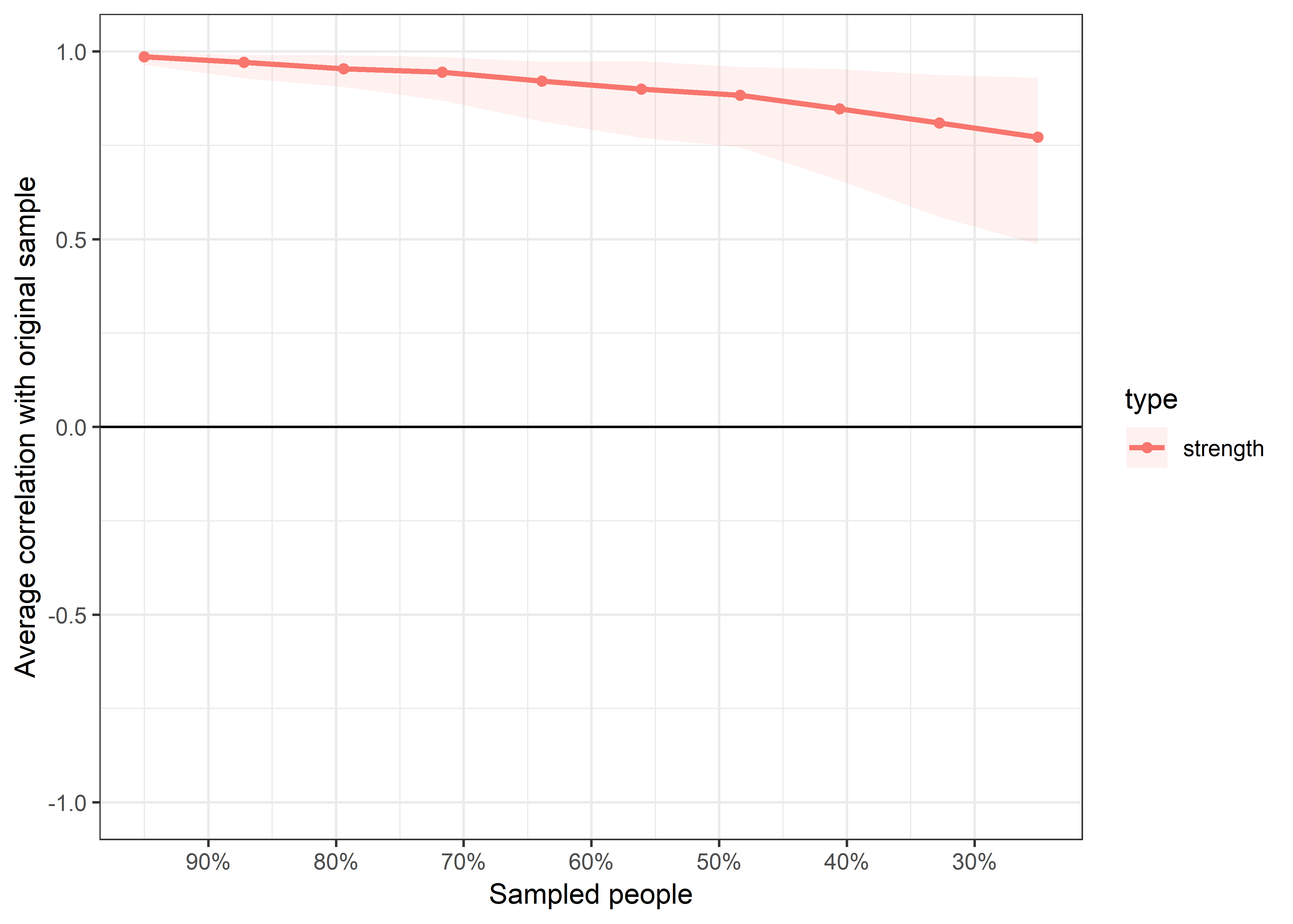
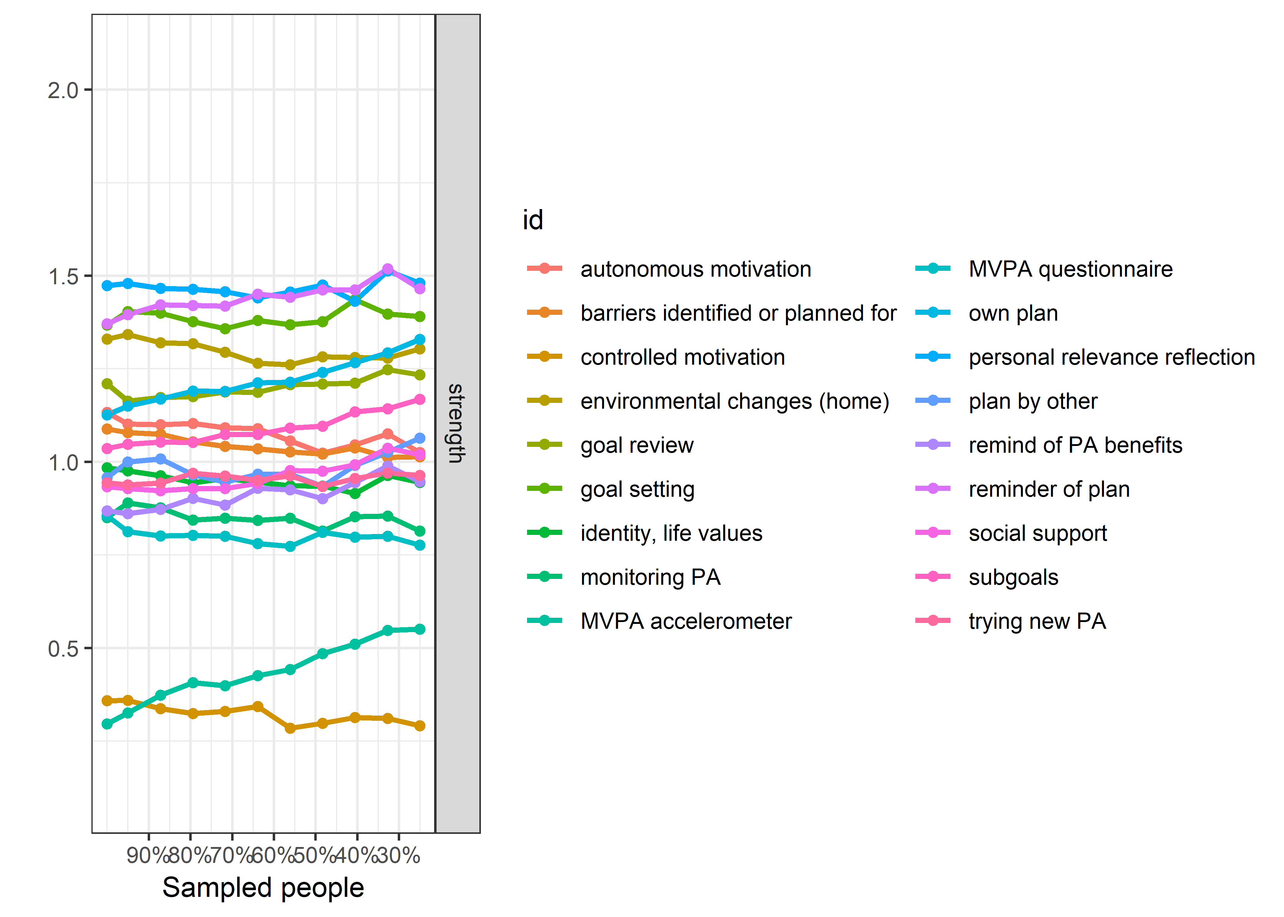
bootnet::corStability(bootnet_centrality_stability_allBctsMotiSurveyPA)
## === Correlation Stability Analysis ===
##
## Sampling levels tested:
##    nPerson Drop%   n
## 1      292  75.0  96
## 2      382  67.2  94
## 3      473  59.4 106
## 4      564  51.6 110
## 5      654  43.9 105
## 6      745  36.1  98
## 7      836  28.3  91
## 8      926  20.6 100
## 9     1017  12.8  97
## 10    1108   5.0 103
##
## Maximum drop proportions to retain correlation of 0.7 in at least 95% of the samples:
##
## edge: 0.75 (CS-coefficient is highest level tested)
##   - For more accuracy, run bootnet(..., caseMin = 0.672, caseMax = 1)
##
## strength: 0.594
##   - For more accuracy, run bootnet(..., caseMin = 0.516, caseMax = 0.672)
##
## Accuracy can also be increased by increasing both 'nBoots' and 'caseN'.
layout_mgm_ggm <- qgraph::averageLayout(BCT_ggm, BCT_mgm)

layout(t(1:2))

plot(nwBCT_ggm, layout = layout_mgm_ggm, label.scale = FALSE, title = "GGM: MVPA, BCTs & motivation", label.cex = 0.75,
     pie = piefill_ggm,
     color = "skyblue",
     pieBorder = 1)

qgraph::qgraph(mgm_obj$pairwise$wadj,
            layout = layout_mgm_ggm,
            title = "MGM: MVPA, BCTs & motivation",
            edge.color = ifelse(mgm_obj$pairwise$edgecolor == "darkgreen", "blue", mgm_obj$pairwise$edgecolor),
            pie = pie_errors,
            pieColor = viridis::viridis(6, begin = 0.3, end = 0.8)[6],
            color = node_colors,
            labels = names(bctdf_mgm),
            label.cex = 0.75,
            label.scale = FALSE)
Correlation and partial correlation networks visualised
As we can see, the bivariate correlation network is uninterpretable due to high number of edges.
corgraph <- qgraph::qgraph(qgraph::cor_auto(bctdf_ggm), graph = "cor",
                           repulsion = 0.99,
       labels = names(bctdf_ggm),
       edge.labels = TRUE,
       edge.label.cex = 0.75,
       label.scale = FALSE,
       layout = qgraph::averageLayout(BCT_ggm, BCT_mgm), # get the mgm layout
       title = "bivariate correlation network",
       theme = "colorblind",
       label.cex = 0.75,
       pie = piefill_ggm,
       pieBorder = 1,
       color = "skyblue")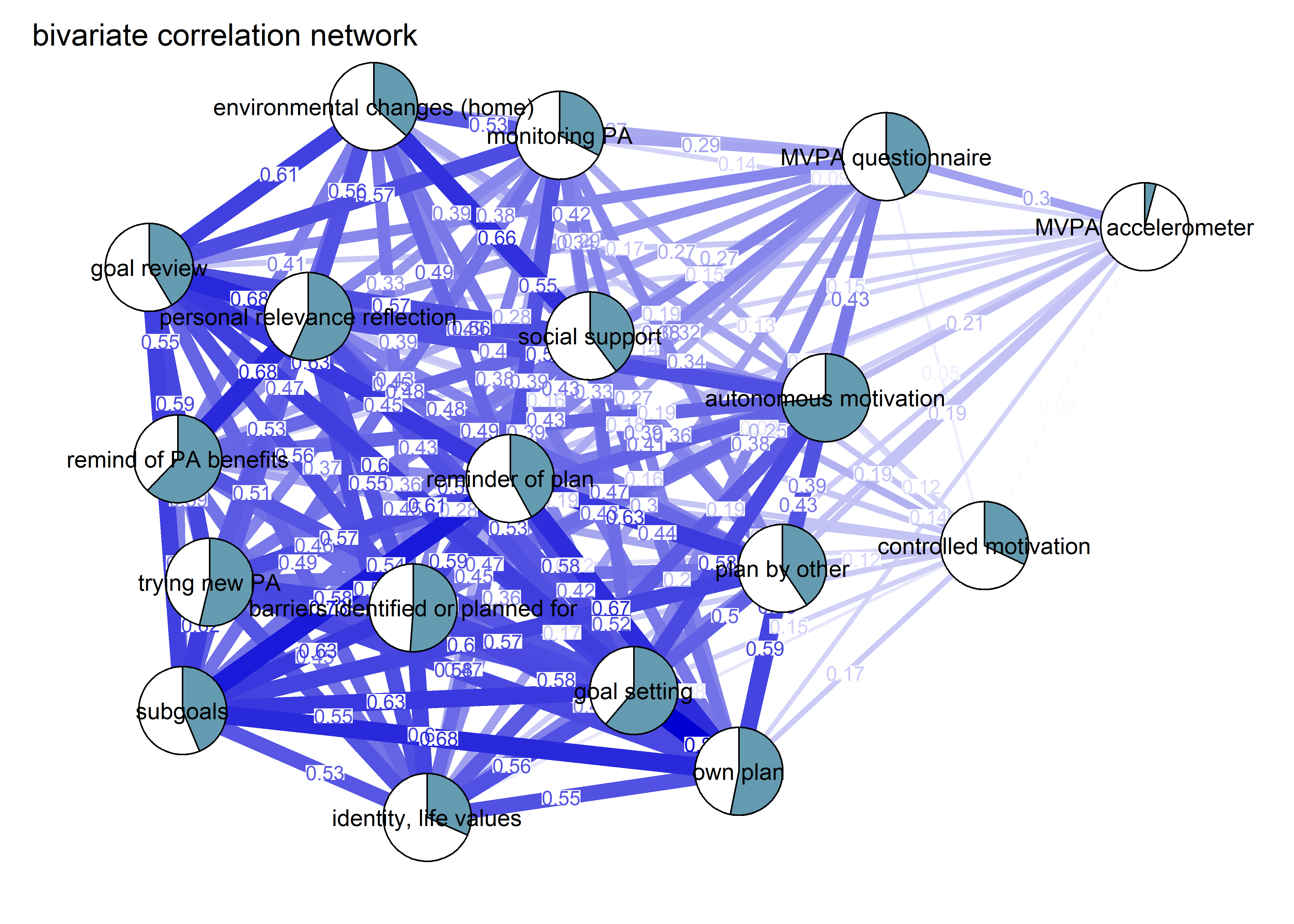
pcorgraph <- qgraph::qgraph(qgraph::cor_auto(bctdf_ggm), graph = "pcor",
                           repulsion = 0.99,
       labels = names(bctdf_ggm),
       edge.labels = TRUE,
       edge.label.cex = 0.75,
       label.scale = FALSE,
       layout = qgraph::averageLayout(BCT_ggm, BCT_mgm), # get the mgm layout
       title = "Partial correlation network",
       theme = "colorblind",
       label.cex = 0.75,
       pie = piefill_ggm,
       pieBorder = 1,
       color = "skyblue")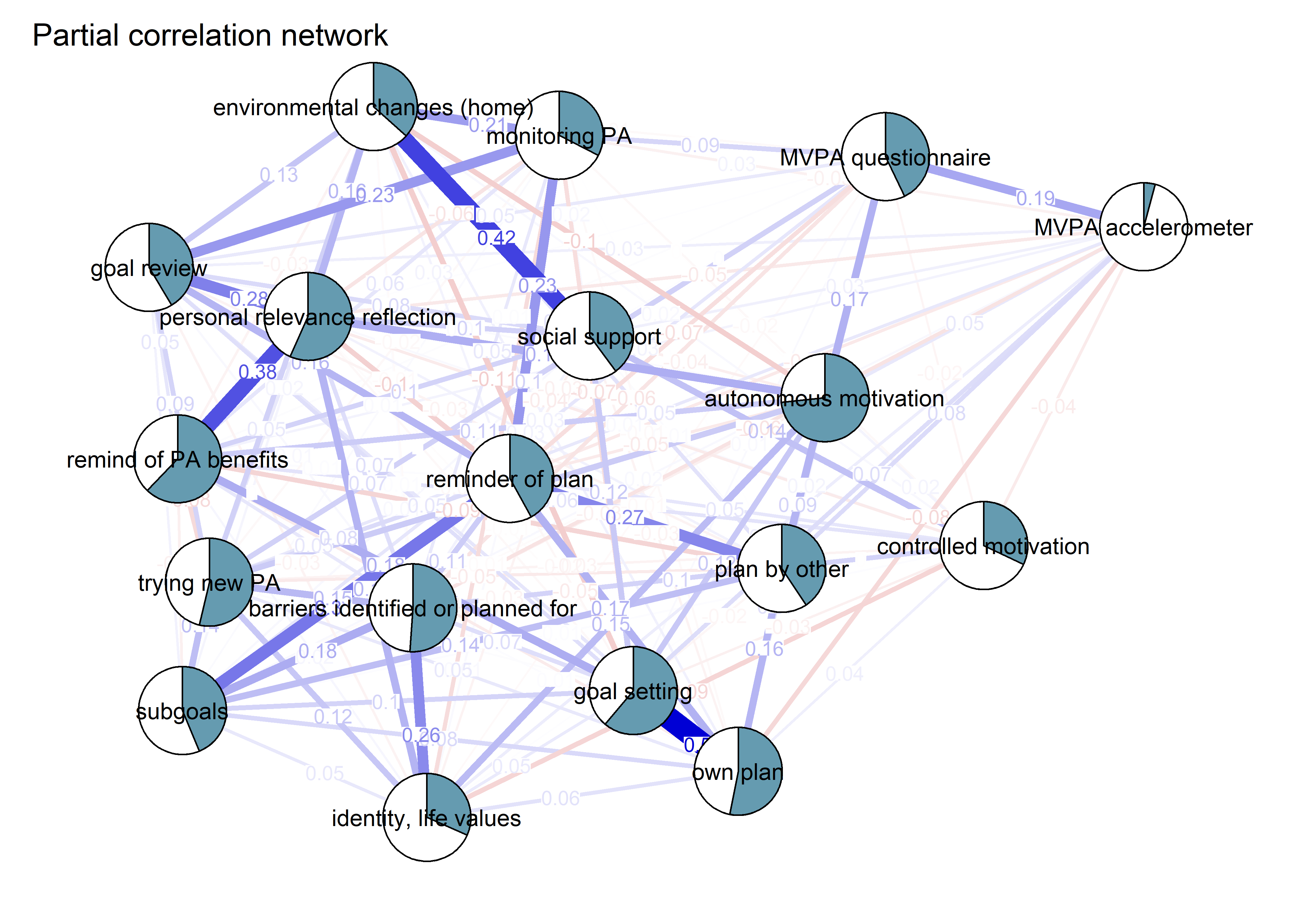
Correlation matrix visualised
bivariate_BCTs <- df %>% dplyr::select(
  'goal setting' = PA_agreementDependentBCT_01_T1,
  'own plan' = PA_agreementDependentBCT_02_T1,
  'plan by other' = PA_agreementDependentBCT_03_T1,
  'reminder of plan' = PA_agreementDependentBCT_04_T1,
  'subgoals' = PA_agreementDependentBCT_05_T1,
  'trying new PA' = PA_agreementDependentBCT_06_T1,
  'barrier identification' = PA_agreementDependentBCT_07_T1,
  'problem solving' = PA_agreementDependentBCT_08_T1,
  'PA identity reflection' = PA_agreementDependentBCT_09_T1,
  'aligning PA with life values' = PA_agreementDependentBCT_10_T1,
  'remind of PA benefits' = PA_frequencyDependentBCT_01_T1,
  'self-monitor (paper)' = PA_frequencyDependentBCT_02_T1,
  'self-monitor (app)' = PA_frequencyDependentBCT_03_T1,
  'memory cues' = PA_frequencyDependentBCT_04_T1,
  'goal review' = PA_frequencyDependentBCT_05_T1,
  'personal relevance reflection' = PA_frequencyDependentBCT_06_T1,
  'environmental changes (home)' = PA_frequencyDependentBCT_07_T1,
  'social support' = PA_frequencyDependentBCT_08_T1,
  'failure contemplated' = PA_frequencyDependentBCT_09_T1,
  'PA accelerometer' = mvpaAccelerometer_T1,
  'PA self-report' = padaysLastweek_T1,
  'autonomous' = PA_autonomous_T1,
  'controlled' = PA_controlled_T1) %>%
 rowwise() %>%
  dplyr::select(`PA accelerometer`, `PA self-report`, autonomous, controlled, everything()) %>%
  mutate_all(as.numeric)

# Create a covariance matrix of the data
covMatrix <- bctdf_ggm %>% cov(use = "pairwise.complete.obs")

# Transform the matrix so, that lower diagonal of the matrix shows partial correlations,
# while the upper one shows bivariate correlations.
matrix_corLower_parcorUpper <- covMatrix %>% ggm::correlations()

# Show the matrix
matrix_corLower_parcorUpper %>% papaja::apa_table(caption = "Correlation matrix of key variables of interest. Lower diagonal shows bivariate correlations, upper diagonal shows partial correlations")| MVPA questionnaire | MVPA accelerometer | autonomous motivation | controlled motivation | goal setting | own plan | plan by other | reminder of plan | subgoals | trying new PA | remind of PA benefits | goal review | personal relevance reflection | environmental changes (home) | social support | barriers identified or planned for | identity, life values | monitoring PA | |
|---|---|---|---|---|---|---|---|---|---|---|---|---|---|---|---|---|---|---|
| MVPA questionnaire | 1.00 | 0.19 | 0.19 | -0.02 | 0.02 | 0.03 | 0.15 | -0.05 | 0.07 | 0.10 | 0.00 | 0.05 | 0.02 | -0.01 | 0.01 | -0.06 | -0.02 | 0.08 |
| MVPA accelerometer | 0.29 | 1.00 | 0.06 | -0.04 | 0.06 | -0.08 | 0.07 | -0.02 | 0.02 | 0.05 | 0.02 | 0.03 | -0.03 | 0.04 | 0.03 | -0.06 | 0.04 | -0.04 |
| autonomous motivation | 0.43 | 0.21 | 1.00 | 0.02 | 0.15 | 0.07 | 0.08 | -0.04 | -0.01 | 0.10 | 0.14 | 0.01 | 0.16 | -0.07 | -0.04 | -0.02 | 0.16 | 0.00 |
| controlled motivation | 0.05 | -0.02 | 0.12 | 1.00 | -0.01 | 0.03 | 0.01 | 0.05 | 0.01 | -0.02 | 0.07 | -0.03 | 0.02 | 0.02 | 0.11 | 0.10 | -0.09 | -0.01 |
| goal setting | 0.35 | 0.17 | 0.54 | 0.14 | 1.00 | 0.49 | -0.01 | -0.01 | 0.06 | 0.00 | 0.14 | 0.05 | -0.01 | -0.04 | 0.07 | 0.09 | 0.05 | -0.06 |
| own plan | 0.36 | 0.12 | 0.51 | 0.16 | 0.74 | 1.00 | 0.13 | 0.15 | 0.11 | 0.05 | -0.03 | 0.07 | -0.01 | 0.01 | 0.00 | 0.03 | 0.07 | -0.02 |
| plan by other | 0.37 | 0.18 | 0.37 | 0.11 | 0.40 | 0.48 | 1.00 | 0.19 | 0.12 | -0.03 | -0.07 | 0.00 | 0.02 | 0.03 | 0.02 | -0.03 | 0.03 | 0.03 |
| reminder of plan | 0.29 | 0.10 | 0.35 | 0.17 | 0.47 | 0.57 | 0.50 | 1.00 | 0.26 | 0.05 | -0.02 | 0.11 | -0.04 | -0.01 | -0.03 | 0.10 | 0.03 | 0.27 |
| subgoals | 0.36 | 0.15 | 0.42 | 0.15 | 0.54 | 0.60 | 0.48 | 0.64 | 1.00 | 0.12 | -0.02 | 0.04 | -0.01 | 0.01 | 0.01 | 0.19 | 0.06 | 0.04 |
| trying new PA | 0.37 | 0.17 | 0.46 | 0.11 | 0.47 | 0.51 | 0.35 | 0.47 | 0.54 | 1.00 | -0.06 | 0.09 | 0.04 | 0.08 | 0.01 | 0.17 | 0.14 | 0.00 |
| remind of PA benefits | 0.27 | 0.13 | 0.47 | 0.18 | 0.47 | 0.40 | 0.23 | 0.31 | 0.35 | 0.34 | 1.00 | 0.05 | 0.34 | 0.00 | 0.09 | 0.06 | 0.04 | 0.04 |
| goal review | 0.36 | 0.16 | 0.43 | 0.14 | 0.50 | 0.53 | 0.39 | 0.55 | 0.53 | 0.50 | 0.46 | 1.00 | 0.21 | 0.09 | 0.09 | 0.04 | -0.01 | 0.25 |
| personal relevance reflection | 0.33 | 0.14 | 0.53 | 0.17 | 0.49 | 0.47 | 0.33 | 0.40 | 0.44 | 0.47 | 0.62 | 0.58 | 1.00 | 0.12 | 0.11 | 0.08 | 0.17 | -0.04 |
| environmental changes (home) | 0.24 | 0.12 | 0.25 | 0.16 | 0.31 | 0.34 | 0.30 | 0.39 | 0.38 | 0.38 | 0.34 | 0.50 | 0.45 | 1.00 | 0.33 | -0.01 | 0.02 | 0.27 |
| social support | 0.24 | 0.12 | 0.30 | 0.22 | 0.38 | 0.37 | 0.29 | 0.35 | 0.37 | 0.35 | 0.41 | 0.48 | 0.48 | 0.56 | 1.00 | 0.04 | -0.02 | 0.05 |
| barriers identified or planned for | 0.27 | 0.09 | 0.43 | 0.20 | 0.54 | 0.55 | 0.37 | 0.54 | 0.60 | 0.56 | 0.44 | 0.52 | 0.53 | 0.37 | 0.40 | 1.00 | 0.25 | 0.04 |
| identity, life values | 0.30 | 0.16 | 0.52 | 0.08 | 0.53 | 0.53 | 0.36 | 0.43 | 0.50 | 0.52 | 0.43 | 0.45 | 0.55 | 0.32 | 0.33 | 0.60 | 1.00 | -0.10 |
| monitoring PA | 0.29 | 0.08 | 0.27 | 0.13 | 0.31 | 0.37 | 0.36 | 0.55 | 0.45 | 0.37 | 0.31 | 0.57 | 0.37 | 0.53 | 0.41 | 0.40 | 0.27 | 1.00 |
labs <- names(bctdf_ggm)
# Plot the matrix as a correlogram
matrix_corLower_parcorUpper %>% corrgram::corrgram(
  type = "cor",
  lower.panel = corrgram::panel.pie,
  upper.panel = corrgram::panel.pie,
  outer.labels = list(bottom = list(labels = labs, cex = 0.75, srt = 30),
                      left = list(labels = labs, cex = 0.75, srt = 30)),
  main = "Bivariate (upper diagonal) and partial (lower diagonal)\ncorrelations of BCTs, motivation and self-reported PA")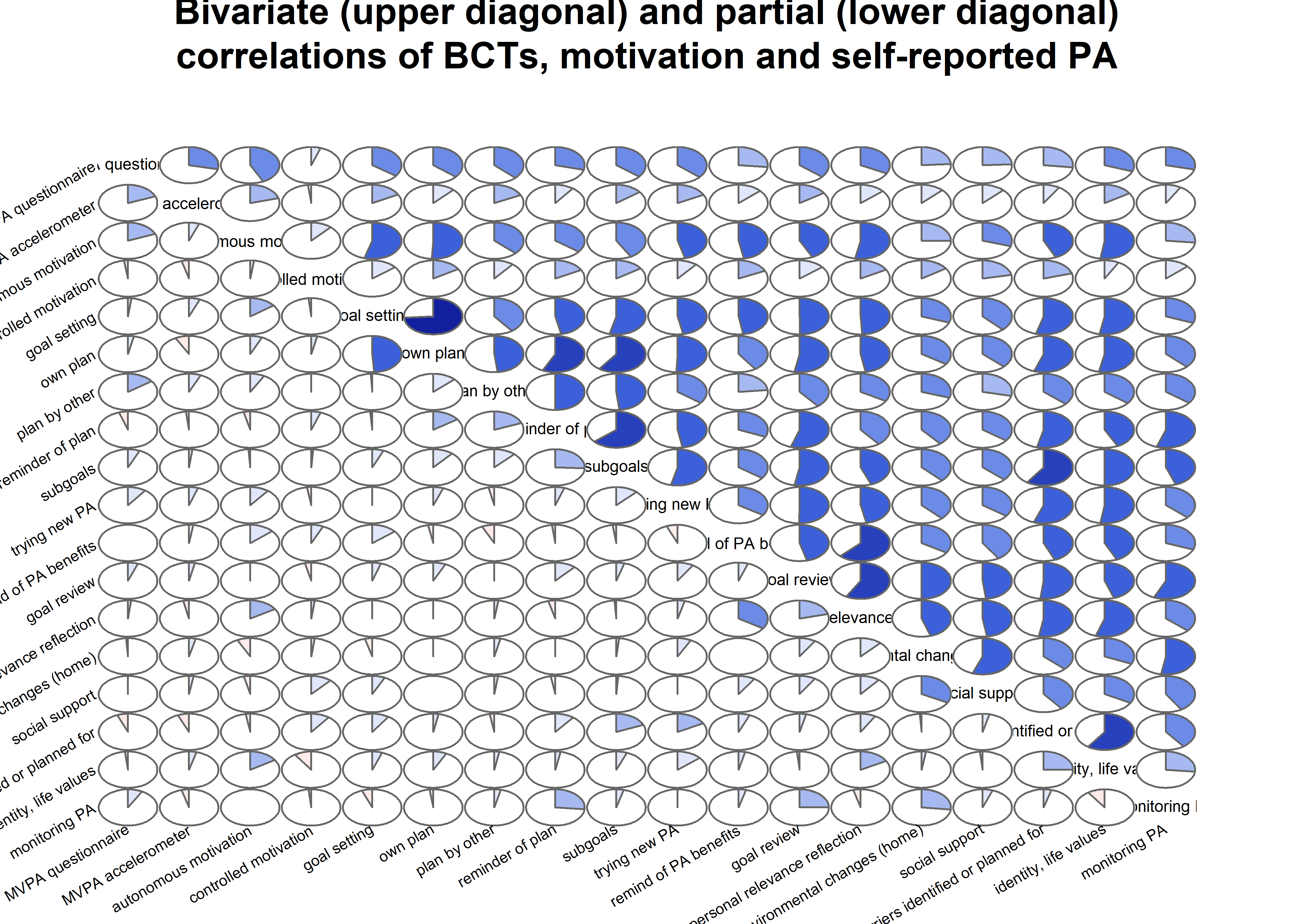
corMatrix_BCTs <- bivariate_BCTs %>% cor(use = "pairwise.complete.obs", method = "spearman")

as.data.frame(as.table(corMatrix_BCTs)) %>%
  dplyr::filter(Var1 == "PA accelerometer" | Var1 == "PA self report") %>%
  dplyr::mutate("Spearman correlation" = Freq) %>%
  dplyr::select(-Freq) %>%
  dplyr::filter(`Spearman correlation` != 1) %>%
  dplyr::arrange(desc(`Spearman correlation`)) %>%
papaja::apa_table(caption = "Bivariate correlations between BCTs, motivation and self-reported PA. Sorted by strength.")| Var1 | Var2 | Spearman correlation |
|---|---|---|
| PA accelerometer | PA accelerometer | 1.00 |
| PA accelerometer | PA self-report | 0.28 |
| PA accelerometer | autonomous | 0.25 |
| PA accelerometer | trying new PA | 0.18 |
| PA accelerometer | goal setting | 0.17 |
| PA accelerometer | aligning PA with life values | 0.16 |
| PA accelerometer | plan by other | 0.16 |
| PA accelerometer | goal review | 0.15 |
| PA accelerometer | subgoals | 0.14 |
| PA accelerometer | social support | 0.13 |
| PA accelerometer | personal relevance reflection | 0.13 |
| PA accelerometer | PA identity reflection | 0.13 |
| PA accelerometer | remind of PA benefits | 0.12 |
| PA accelerometer | own plan | 0.11 |
| PA accelerometer | environmental changes (home) | 0.11 |
| PA accelerometer | failure contemplated | 0.10 |
| PA accelerometer | self-monitor (paper) | 0.09 |
| PA accelerometer | reminder of plan | 0.09 |
| PA accelerometer | barrier identification | 0.08 |
| PA accelerometer | memory cues | 0.08 |
| PA accelerometer | problem solving | 0.06 |
| PA accelerometer | self-monitor (app) | 0.04 |
| PA accelerometer | controlled | -0.03 |
Cognitive BCTs only, added one at a time
Four BCTs can be categorised as being completely cognitive, i.e. not being observable to an outsider. These are (in order of correlation with accelerometer-measured MVPA:
- I have attempted to find ways to exercise so, that it won’t obstruct but instead helps actualise my other life values.
- I have thought about which reasons to do PA are important to me personally.
- I have reminded myself even in my spare time, what kind of positive consequences frequent PA would have in my life.
- I have thought about how PA fits my identity (self concept).
First, we fit a model with only the first one:
bctdf_mgm <- df %>% dplyr::select(
#  id,
#  intervention,
#  group,
#  school,
#  girl,
  'goal setting' = PA_agreementDependentBCT_01_T1,
  'own plan' = PA_agreementDependentBCT_02_T1,
  'plan by other' = PA_agreementDependentBCT_03_T1,
  'reminder of plan' = PA_agreementDependentBCT_04_T1,
  'subgoals' = PA_agreementDependentBCT_05_T1,
  'trying new PA' = PA_agreementDependentBCT_06_T1,
  'barrier identification' = PA_agreementDependentBCT_07_T1,
  'problem solving' = PA_agreementDependentBCT_08_T1,
  'PA identity reflection' = PA_agreementDependentBCT_09_T1,
  'aligning PA with life values' = PA_agreementDependentBCT_10_T1,
  'remind of PA benefits' = PA_frequencyDependentBCT_01_T1,
  'self-monitor (paper)' = PA_frequencyDependentBCT_02_T1,
  'self-monitor (app)' = PA_frequencyDependentBCT_03_T1,
#  'memory cues' = PA_frequencyDependentBCT_04_T1, # Issues with clarity of item wording
  'goal review' = PA_frequencyDependentBCT_05_T1,
  'personal relevance reflection' = PA_frequencyDependentBCT_06_T1,
  'environmental changes (home)' = PA_frequencyDependentBCT_07_T1,
  'social support' = PA_frequencyDependentBCT_08_T1,
  'analysing goal failure' = PA_frequencyDependentBCT_09_T1,
  'MVPA questionnaire' = padaysLastweek_T1,
  'MVPA accelerometer' = mvpaAccelerometer_T1,
  'intrinsic' = PA_intrinsic_T1,
  'identified' = PA_identified_T1,
  'controlled motivation' = PA_controlled_T1) %>%
 rowwise() %>%
 dplyr::transmute(
  # 'goal setting' = ifelse(`goal setting` == 1, 0, 1),
  # 'has plan' = ifelse(`own plan` == 1 & `plan by other` == 1, 0, 1),
  # 'own plan' = ifelse(`own plan` == 1, 0, 1),
  # 'plan by other' = ifelse(`plan by other` == 1, 0, 1),
  # 'reminder of plan' = ifelse(`reminder of plan` == 1, 0, 1),
  # 'subgoals' = ifelse(`subgoals` == 1, 0, 1),
  # 'trying new PA' = ifelse(`trying new PA` == 1, 0, 1),
  # 'barrier identification' = ifelse(`barrier identification` == 1, 0, 1),
  # 'problem solving' = ifelse(`problem solving` == 1, 0, 1),
  # 'barriers identified or planned for' = ifelse(`problem solving` == 1 & `barrier identification` == 1, 0, 1),
 # 'PA identity reflection' = ifelse(`PA identity reflection` == 1, 0, 1),
 'aligning PA with life values' = ifelse(`aligning PA with life values` == 1, 0, 1),
  # 'identity, life values' = ifelse(`PA identity reflection` == 1 & `aligning PA with life values` == 1, 0, 1),
  # 'remind of PA benefits' = ifelse(`remind of PA benefits` == 1, 0, 1),
  # 'monitoring PA' = ifelse(`self-monitor (paper)` == 1 & `self-monitor (app)` == 1, 0, 1),
  # 'memory cues' = ifelse(`memory cues` == 1, 0, 1),
  # 'goal review' = ifelse(`goal review` == 1, 0, 1),
  # 'personal relevance reflection' = ifelse(`personal relevance reflection` == 1, 0, 1),
  # 'environmental changes (home)' = ifelse(`environmental changes (home)` == 1, 0, 1),
  # 'social support' = ifelse(`social support` == 1, 0, 1),
  # 'analysing goal failure' = ifelse(`analysing goal failure` == 1, 0, 1),
  'autonomous motivation' = mean(c(identified, intrinsic), na.rm = TRUE),
#  'girl' = ifelse(girl == "girl", 1, 0),
  'controlled motivation' = ifelse(`controlled motivation` < 3, 0, 1), # If "at least partly" or more true, input 1. Normality otherwise a problem.
  'MVPA questionnaire' = `MVPA questionnaire` * 1,
  'MVPA accelerometer' = `MVPA accelerometer` * 1) %>%
  dplyr::select('MVPA questionnaire', 'MVPA accelerometer', everything())

bctdf_mgm$`autonomous motivation`[is.nan(bctdf_mgm$`autonomous motivation`)] <- NA

labs <- names(bctdf_mgm)

bctdf_mgm <- bctdf_mgm %>% na.omit(.)
# bctdf_mgm %>% names()
mgm_variable_types <- c("g", "g", rep("c", 1), "g", "c")
mgm_variable_levels <- c("1", "1", rep("2", 1), "1", "2")
# data.frame(mgm_variable_types, mgm_variable_levels, names(bctdf_mgm))

mgm_obj <- mgm::mgm(data = bctdf_mgm,
  type = mgm_variable_types,
  level = mgm_variable_levels,
  lambdaSel = "CV",
  lambdaFolds = 10,
  pbar = FALSE,
  binarySign = TRUE)
## Note that the sign of parameter estimates is stored separately; see ?mgm

pred_obj <- predict(object = mgm_obj,
                         data = bctdf_mgm)

pred_obj$errors
# Take R2 from gaussian, CC from categorical variables
pie_errors <- c(pred_obj$errors[1, 3],
                pred_obj$errors[2, 3],
                pred_obj$errors[3, 4],
                pred_obj$errors[4, 3],
                pred_obj$errors[5, 4])

# Coloring nodes: make a sequence of colors from the viridis palette. We need three colors (MVPA, BCTs, motivation), and "begin" from ones that are not too dark, so that black text shows up ok.

node_colors <- c(viridis::viridis(3, begin = 0.4, end = 0.99)[1], # Color 1 for MVPA (questionnaire)
                 viridis::viridis(3, begin = 0.4, end = 0.99)[1], # Color 1 for MVPA (accelerometer)
                 rep(viridis::viridis(3, begin = 0.4, end = 0.99)[2], 1), # 4x Color 2 for BCTs
                 rep(viridis::viridis(3, begin = 0.4, end = 0.99)[3], 1), # Color 3 for motivation (controlled)
                 viridis::viridis(3, begin = 0.4, end = 0.99)[3]) # Color 3 for motivation (autonomous)

BCT_mgm <- qgraph::qgraph(mgm_obj$pairwise$wadj,
            layout = "spring",
            repulsion = 0.99, # To nudge the network from originally bad visual state
            title = "cognitive/motivational BCTs, PA & motivation",
            edge.color = ifelse(mgm_obj$pairwise$edgecolor == "darkgreen", "blue", mgm_obj$pairwise$edgecolor),
            pie = pie_errors,
            pieColor = viridis::viridis(5, begin = 0.3, end = 0.8)[5],
            color = node_colors,
            labels = names(bctdf_mgm),
            label.cex = 0.75,
            label.scale = FALSE,
            vertex.label.dist = 2)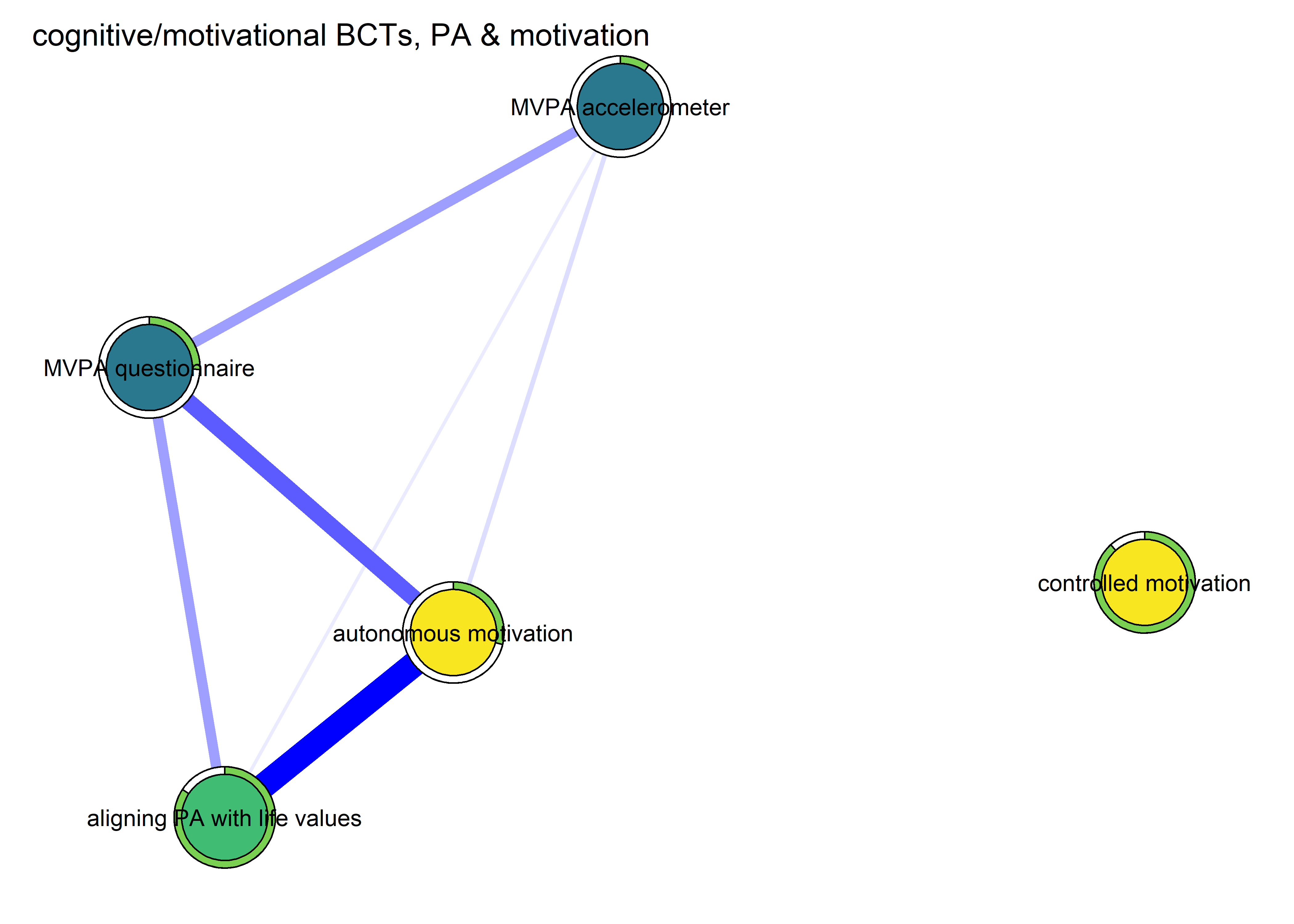
Adding the second (I have thought about which reasons to do PA are important to me personally):
bctdf_mgm <- df %>% dplyr::select(
#  id,
#  intervention,
#  group,
#  school,
#  girl,
  'goal setting' = PA_agreementDependentBCT_01_T1,
  'own plan' = PA_agreementDependentBCT_02_T1,
  'plan by other' = PA_agreementDependentBCT_03_T1,
  'reminder of plan' = PA_agreementDependentBCT_04_T1,
  'subgoals' = PA_agreementDependentBCT_05_T1,
  'trying new PA' = PA_agreementDependentBCT_06_T1,
  'barrier identification' = PA_agreementDependentBCT_07_T1,
  'problem solving' = PA_agreementDependentBCT_08_T1,
  'PA identity reflection' = PA_agreementDependentBCT_09_T1,
  'aligning PA with life values' = PA_agreementDependentBCT_10_T1,
  'remind of PA benefits' = PA_frequencyDependentBCT_01_T1,
  'self-monitor (paper)' = PA_frequencyDependentBCT_02_T1,
  'self-monitor (app)' = PA_frequencyDependentBCT_03_T1,
#  'memory cues' = PA_frequencyDependentBCT_04_T1, # Issues with clarity of item wording
  'goal review' = PA_frequencyDependentBCT_05_T1,
  'personal relevance reflection' = PA_frequencyDependentBCT_06_T1,
  'environmental changes (home)' = PA_frequencyDependentBCT_07_T1,
  'social support' = PA_frequencyDependentBCT_08_T1,
  'analysing goal failure' = PA_frequencyDependentBCT_09_T1,
  'MVPA questionnaire' = padaysLastweek_T1,
  'MVPA accelerometer' = mvpaAccelerometer_T1,
  'intrinsic' = PA_intrinsic_T1,
  'identified' = PA_identified_T1,
  'controlled motivation' = PA_controlled_T1) %>%
 rowwise() %>%
 dplyr::transmute(
  # 'goal setting' = ifelse(`goal setting` == 1, 0, 1),
  # 'has plan' = ifelse(`own plan` == 1 & `plan by other` == 1, 0, 1),
  # 'own plan' = ifelse(`own plan` == 1, 0, 1),
  # 'plan by other' = ifelse(`plan by other` == 1, 0, 1),
  # 'reminder of plan' = ifelse(`reminder of plan` == 1, 0, 1),
  # 'subgoals' = ifelse(`subgoals` == 1, 0, 1),
  # 'trying new PA' = ifelse(`trying new PA` == 1, 0, 1),
  # 'barrier identification' = ifelse(`barrier identification` == 1, 0, 1),
  # 'problem solving' = ifelse(`problem solving` == 1, 0, 1),
  # 'barriers identified or planned for' = ifelse(`problem solving` == 1 & `barrier identification` == 1, 0, 1),
 # 'PA identity reflection' = ifelse(`PA identity reflection` == 1, 0, 1),
 'aligning PA with life values' = ifelse(`aligning PA with life values` == 1, 0, 1),
  # 'identity, life values' = ifelse(`PA identity reflection` == 1 & `aligning PA with life values` == 1, 0, 1),
  # 'remind of PA benefits' = ifelse(`remind of PA benefits` == 1, 0, 1),
  # 'monitoring PA' = ifelse(`self-monitor (paper)` == 1 & `self-monitor (app)` == 1, 0, 1),
  # 'memory cues' = ifelse(`memory cues` == 1, 0, 1),
  # 'goal review' = ifelse(`goal review` == 1, 0, 1),
  'personal relevance reflection' = ifelse(`personal relevance reflection` == 1, 0, 1),
  # 'environmental changes (home)' = ifelse(`environmental changes (home)` == 1, 0, 1),
  # 'social support' = ifelse(`social support` == 1, 0, 1),
  # 'analysing goal failure' = ifelse(`analysing goal failure` == 1, 0, 1),
  'autonomous motivation' = mean(c(identified, intrinsic), na.rm = TRUE),
#  'girl' = ifelse(girl == "girl", 1, 0),
  'controlled motivation' = ifelse(`controlled motivation` < 3, 0, 1), # If "at least partly" or more true, input 1. Normality otherwise a problem.
  'MVPA questionnaire' = `MVPA questionnaire` * 1,
  'MVPA accelerometer' = `MVPA accelerometer` * 1) %>%
  dplyr::select('MVPA questionnaire', 'MVPA accelerometer', everything())

bctdf_mgm$`autonomous motivation`[is.nan(bctdf_mgm$`autonomous motivation`)] <- NA

labs <- names(bctdf_mgm)

bctdf_mgm <- bctdf_mgm %>% na.omit(.)
# bctdf_mgm %>% names()
mgm_variable_types <- c("g", "g", rep("c", 2), "g", "c")
mgm_variable_levels <- c("1", "1", rep("2", 2), "1", "2")
# data.frame(mgm_variable_types, mgm_variable_levels, names(bctdf_mgm))

mgm_obj <- mgm::mgm(data = bctdf_mgm,
  type = mgm_variable_types,
  level = mgm_variable_levels,
  lambdaSel = "CV",
  lambdaFolds = 10,
  pbar = FALSE,
  binarySign = TRUE)
## Note that the sign of parameter estimates is stored separately; see ?mgm

pred_obj <- predict(object = mgm_obj,
                         data = bctdf_mgm)

pred_obj$errors
# Take R2 from gaussian, CC from categorical variables
pie_errors <- c(pred_obj$errors[1, 3],
                pred_obj$errors[2, 3],
                pred_obj$errors[3:4, 4],
                pred_obj$errors[5, 3],
                pred_obj$errors[6, 4])

# Coloring nodes: make a sequence of colors from the viridis palette. We need three colors (MVPA, BCTs, motivation), and "begin" from ones that are not too dark, so that black text shows up ok.

node_colors <- c(viridis::viridis(3, begin = 0.4, end = 0.99)[1], # Color 1 for MVPA (questionnaire)
                 viridis::viridis(3, begin = 0.4, end = 0.99)[1], # Color 1 for MVPA (accelerometer)
                 rep(viridis::viridis(3, begin = 0.4, end = 0.99)[2], 2), # 2x Color 2 for BCTs
                 rep(viridis::viridis(3, begin = 0.4, end = 0.99)[3], 1), # Color 3 for motivation (controlled)
                 viridis::viridis(3, begin = 0.4, end = 0.99)[3]) # Color 3 for motivation (autonomous)

BCT_mgm <- qgraph::qgraph(mgm_obj$pairwise$wadj,
            layout = "spring",
            repulsion = 0.99, # To nudge the network from originally bad visual state
            title = "cognitive/motivational BCTs, PA & motivation",
            edge.color = ifelse(mgm_obj$pairwise$edgecolor == "darkgreen", "blue", mgm_obj$pairwise$edgecolor),
            pie = pie_errors,
            pieColor = viridis::viridis(5, begin = 0.3, end = 0.8)[5],
            color = node_colors,
            labels = names(bctdf_mgm),
            label.cex = 0.75,
            label.scale = FALSE)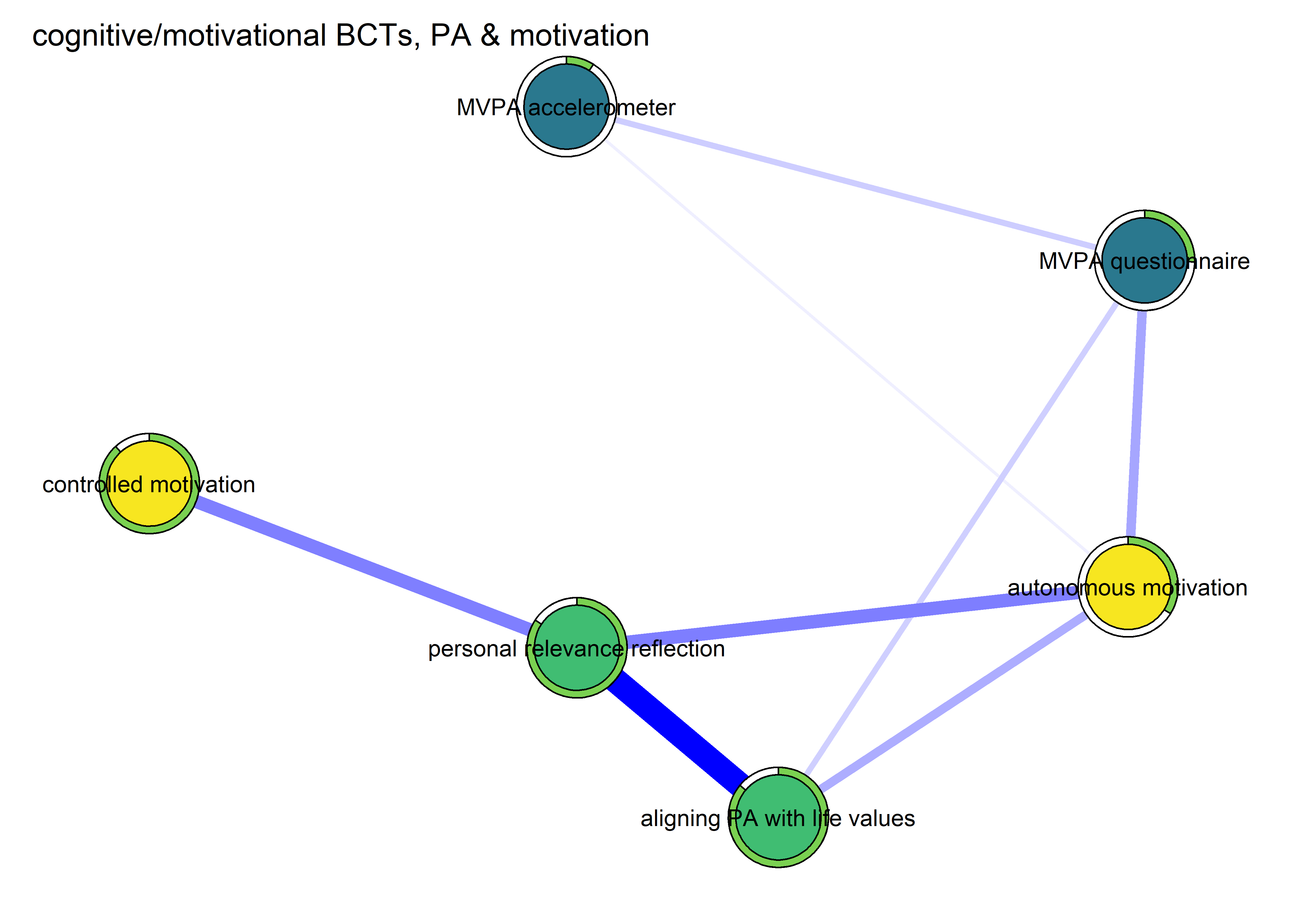
Adding the third (I have reminded myself even in my spare time, what kind of positive consequences frequent PA would have in my life):
bctdf_mgm <- df %>% dplyr::select(
#  id,
#  intervention,
#  group,
#  school,
#  girl,
  'goal setting' = PA_agreementDependentBCT_01_T1,
  'own plan' = PA_agreementDependentBCT_02_T1,
  'plan by other' = PA_agreementDependentBCT_03_T1,
  'reminder of plan' = PA_agreementDependentBCT_04_T1,
  'subgoals' = PA_agreementDependentBCT_05_T1,
  'trying new PA' = PA_agreementDependentBCT_06_T1,
  'barrier identification' = PA_agreementDependentBCT_07_T1,
  'problem solving' = PA_agreementDependentBCT_08_T1,
  'PA identity reflection' = PA_agreementDependentBCT_09_T1,
  'aligning PA with life values' = PA_agreementDependentBCT_10_T1,
  'remind of PA benefits' = PA_frequencyDependentBCT_01_T1,
  'self-monitor (paper)' = PA_frequencyDependentBCT_02_T1,
  'self-monitor (app)' = PA_frequencyDependentBCT_03_T1,
#  'memory cues' = PA_frequencyDependentBCT_04_T1, # Issues with clarity of item wording
  'goal review' = PA_frequencyDependentBCT_05_T1,
  'personal relevance reflection' = PA_frequencyDependentBCT_06_T1,
  'environmental changes (home)' = PA_frequencyDependentBCT_07_T1,
  'social support' = PA_frequencyDependentBCT_08_T1,
  'analysing goal failure' = PA_frequencyDependentBCT_09_T1,
  'MVPA questionnaire' = padaysLastweek_T1,
  'MVPA accelerometer' = mvpaAccelerometer_T1,
  'intrinsic' = PA_intrinsic_T1,
  'identified' = PA_identified_T1,
  'controlled motivation' = PA_controlled_T1) %>%
 rowwise() %>%
 dplyr::transmute(
  # 'goal setting' = ifelse(`goal setting` == 1, 0, 1),
  # 'has plan' = ifelse(`own plan` == 1 & `plan by other` == 1, 0, 1),
  # 'own plan' = ifelse(`own plan` == 1, 0, 1),
  # 'plan by other' = ifelse(`plan by other` == 1, 0, 1),
  # 'reminder of plan' = ifelse(`reminder of plan` == 1, 0, 1),
  # 'subgoals' = ifelse(`subgoals` == 1, 0, 1),
  # 'trying new PA' = ifelse(`trying new PA` == 1, 0, 1),
  # 'barrier identification' = ifelse(`barrier identification` == 1, 0, 1),
  # 'problem solving' = ifelse(`problem solving` == 1, 0, 1),
  # 'barriers identified or planned for' = ifelse(`problem solving` == 1 & `barrier identification` == 1, 0, 1),
 # 'PA identity reflection' = ifelse(`PA identity reflection` == 1, 0, 1),
 'aligning PA with life values' = ifelse(`aligning PA with life values` == 1, 0, 1),
  # 'identity, life values' = ifelse(`PA identity reflection` == 1 & `aligning PA with life values` == 1, 0, 1),
  'remind of PA benefits' = ifelse(`remind of PA benefits` == 1, 0, 1),
  # 'monitoring PA' = ifelse(`self-monitor (paper)` == 1 & `self-monitor (app)` == 1, 0, 1),
  # 'memory cues' = ifelse(`memory cues` == 1, 0, 1),
  # 'goal review' = ifelse(`goal review` == 1, 0, 1),
  'personal relevance reflection' = ifelse(`personal relevance reflection` == 1, 0, 1),
  # 'environmental changes (home)' = ifelse(`environmental changes (home)` == 1, 0, 1),
  # 'social support' = ifelse(`social support` == 1, 0, 1),
  # 'analysing goal failure' = ifelse(`analysing goal failure` == 1, 0, 1),
  'autonomous motivation' = mean(c(identified, intrinsic), na.rm = TRUE),
#  'girl' = ifelse(girl == "girl", 1, 0),
  'controlled motivation' = ifelse(`controlled motivation` < 3, 0, 1), # If "at least partly" or more true, input 1. Normality otherwise a problem.
  'MVPA questionnaire' = `MVPA questionnaire` * 1,
  'MVPA accelerometer' = `MVPA accelerometer` * 1) %>%
  dplyr::select('MVPA questionnaire', 'MVPA accelerometer', everything())

bctdf_mgm$`autonomous motivation`[is.nan(bctdf_mgm$`autonomous motivation`)] <- NA

labs <- names(bctdf_mgm)

bctdf_mgm <- bctdf_mgm %>% na.omit(.)
# bctdf_mgm %>% names()
mgm_variable_types <- c("g", "g", rep("c", 3), "g", "c")
mgm_variable_levels <- c("1", "1", rep("2", 3), "1", "2")
# data.frame(mgm_variable_types, mgm_variable_levels, names(bctdf_mgm))

mgm_obj <- mgm::mgm(data = bctdf_mgm,
  type = mgm_variable_types,
  level = mgm_variable_levels,
  lambdaSel = "CV",
  lambdaFolds = 10,
  pbar = FALSE,
  binarySign = TRUE)
## Note that the sign of parameter estimates is stored separately; see ?mgm

pred_obj <- predict(object = mgm_obj,
                         data = bctdf_mgm)

pred_obj$errors
# Take R2 from gaussian, CC from categorical variables
pie_errors <- c(pred_obj$errors[1, 3],
                pred_obj$errors[2, 3],
                pred_obj$errors[3:5, 4],
                pred_obj$errors[6, 3],
                pred_obj$errors[7, 4])

# Coloring nodes: make a sequence of colors from the viridis palette. We need three colors (MVPA, BCTs, motivation), and "begin" from ones that are not too dark, so that black text shows up ok.

node_colors <- c(viridis::viridis(3, begin = 0.4, end = 0.99)[1], # Color 1 for MVPA (questionnaire)
                 viridis::viridis(3, begin = 0.4, end = 0.99)[1], # Color 1 for MVPA (accelerometer)
                 rep(viridis::viridis(3, begin = 0.4, end = 0.99)[2], 3), # 3x Color 2 for BCTs
                 rep(viridis::viridis(3, begin = 0.4, end = 0.99)[3], 1), # Color 3 for motivation (controlled)
                 viridis::viridis(3, begin = 0.4, end = 0.99)[3]) # Color 3 for motivation (autonomous)

BCT_mgm <- qgraph::qgraph(mgm_obj$pairwise$wadj,
            layout = "spring",
            repulsion = 0.99, # To nudge the network from originally bad visual state
            title = "cognitive/motivational BCTs, PA & motivation",
            edge.color = ifelse(mgm_obj$pairwise$edgecolor == "darkgreen", "blue", mgm_obj$pairwise$edgecolor),
            pie = pie_errors,
            pieColor = viridis::viridis(5, begin = 0.3, end = 0.8)[5],
            color = node_colors,
            labels = names(bctdf_mgm),
            label.cex = 0.75,
            label.scale = FALSE)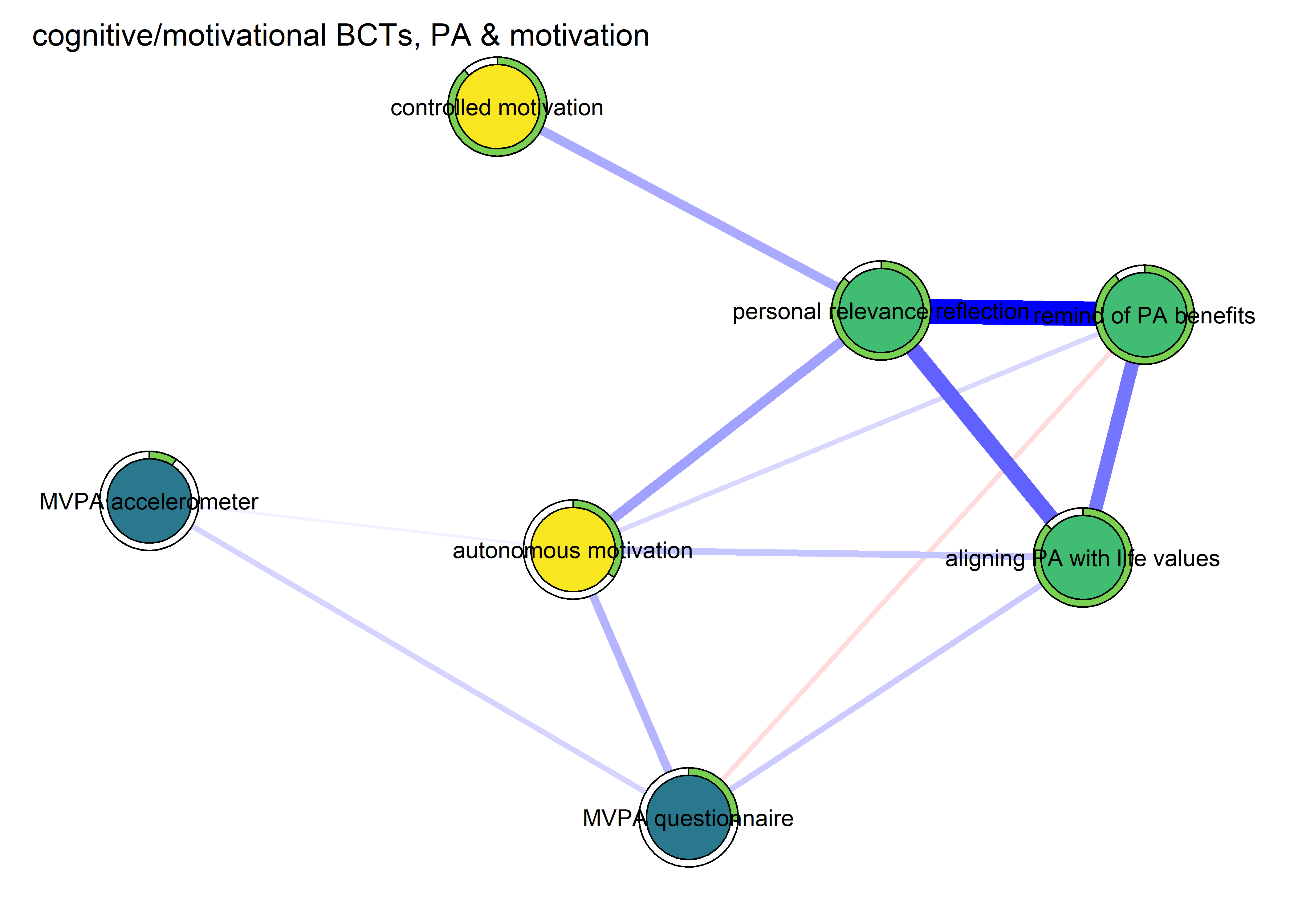
Adding the fourth (I have thought about how PA fits my identity (self concept)):
bctdf_mgm <- df %>% dplyr::select(
#  id,
#  intervention,
#  group,
#  school,
#  girl,
  'goal setting' = PA_agreementDependentBCT_01_T1,
  'own plan' = PA_agreementDependentBCT_02_T1,
  'plan by other' = PA_agreementDependentBCT_03_T1,
  'reminder of plan' = PA_agreementDependentBCT_04_T1,
  'subgoals' = PA_agreementDependentBCT_05_T1,
  'trying new PA' = PA_agreementDependentBCT_06_T1,
  'barrier identification' = PA_agreementDependentBCT_07_T1,
  'problem solving' = PA_agreementDependentBCT_08_T1,
  'PA identity reflection' = PA_agreementDependentBCT_09_T1,
  'aligning PA with life values' = PA_agreementDependentBCT_10_T1,
  'remind of PA benefits' = PA_frequencyDependentBCT_01_T1,
  'self-monitor (paper)' = PA_frequencyDependentBCT_02_T1,
  'self-monitor (app)' = PA_frequencyDependentBCT_03_T1,
#  'memory cues' = PA_frequencyDependentBCT_04_T1, # Issues with clarity of item wording
  'goal review' = PA_frequencyDependentBCT_05_T1,
  'personal relevance reflection' = PA_frequencyDependentBCT_06_T1,
  'environmental changes (home)' = PA_frequencyDependentBCT_07_T1,
  'social support' = PA_frequencyDependentBCT_08_T1,
  'analysing goal failure' = PA_frequencyDependentBCT_09_T1,
  'MVPA questionnaire' = padaysLastweek_T1,
  'MVPA accelerometer' = mvpaAccelerometer_T1,
  'intrinsic' = PA_intrinsic_T1,
  'identified' = PA_identified_T1,
  'controlled motivation' = PA_controlled_T1) %>%
 rowwise() %>%
 dplyr::transmute(
  # 'goal setting' = ifelse(`goal setting` == 1, 0, 1),
  # 'has plan' = ifelse(`own plan` == 1 & `plan by other` == 1, 0, 1),
  # 'own plan' = ifelse(`own plan` == 1, 0, 1),
  # 'plan by other' = ifelse(`plan by other` == 1, 0, 1),
  # 'reminder of plan' = ifelse(`reminder of plan` == 1, 0, 1),
  # 'subgoals' = ifelse(`subgoals` == 1, 0, 1),
  # 'trying new PA' = ifelse(`trying new PA` == 1, 0, 1),
  # 'barrier identification' = ifelse(`barrier identification` == 1, 0, 1),
  # 'problem solving' = ifelse(`problem solving` == 1, 0, 1),
  # 'barriers identified or planned for' = ifelse(`problem solving` == 1 & `barrier identification` == 1, 0, 1),
 'PA identity reflection' = ifelse(`PA identity reflection` == 1, 0, 1),
 'aligning PA with life values' = ifelse(`aligning PA with life values` == 1, 0, 1),
  # 'identity, life values' = ifelse(`PA identity reflection` == 1 & `aligning PA with life values` == 1, 0, 1),
  'remind of PA benefits' = ifelse(`remind of PA benefits` == 1, 0, 1),
  # 'monitoring PA' = ifelse(`self-monitor (paper)` == 1 & `self-monitor (app)` == 1, 0, 1),
  # 'memory cues' = ifelse(`memory cues` == 1, 0, 1),
  # 'goal review' = ifelse(`goal review` == 1, 0, 1),
  'personal relevance reflection' = ifelse(`personal relevance reflection` == 1, 0, 1),
  # 'environmental changes (home)' = ifelse(`environmental changes (home)` == 1, 0, 1),
  # 'social support' = ifelse(`social support` == 1, 0, 1),
  # 'analysing goal failure' = ifelse(`analysing goal failure` == 1, 0, 1),
  'autonomous motivation' = mean(c(identified, intrinsic), na.rm = TRUE),
#  'girl' = ifelse(girl == "girl", 1, 0),
  'controlled motivation' = ifelse(`controlled motivation` < 3, 0, 1), # If "at least partly" or more true, input 1. Normality otherwise a problem.
  'MVPA questionnaire' = `MVPA questionnaire` * 1,
  'MVPA accelerometer' = `MVPA accelerometer` * 1) %>%
  dplyr::select('MVPA questionnaire', 'MVPA accelerometer', everything())

bctdf_mgm$`autonomous motivation`[is.nan(bctdf_mgm$`autonomous motivation`)] <- NA

labs <- names(bctdf_mgm)

bctdf_mgm <- bctdf_mgm %>% na.omit(.)
# bctdf_mgm %>% names()
mgm_variable_types <- c("g", "g", rep("c", 4), "g", "c")
mgm_variable_levels <- c("1", "1", rep("2", 4), "1", "2")
# data.frame(mgm_variable_types, mgm_variable_levels, names(bctdf_mgm))

mgm_obj <- mgm::mgm(data = bctdf_mgm,
  type = mgm_variable_types,
  level = mgm_variable_levels,
  lambdaSel = "CV",
  lambdaFolds = 10,
  pbar = FALSE,
  binarySign = TRUE)
## Note that the sign of parameter estimates is stored separately; see ?mgm

pred_obj <- predict(object = mgm_obj,
                         data = bctdf_mgm)

pred_obj$errors
# Take R2 from gaussian, CC from categorical variables
pie_errors <- c(pred_obj$errors[1, 3],
                pred_obj$errors[2, 3],
                pred_obj$errors[3:6, 4],
                pred_obj$errors[7, 3],
                pred_obj$errors[8, 4])

# Coloring nodes: make a sequence of colors from the viridis palette. We need three colors (MVPA, BCTs, motivation), and "begin" from ones that are not too dark, so that black text shows up ok.

node_colors <- c(viridis::viridis(3, begin = 0.4, end = 0.99)[1], # Color 1 for MVPA (questionnaire)
                 viridis::viridis(3, begin = 0.4, end = 0.99)[1], # Color 1 for MVPA (accelerometer)
                 rep(viridis::viridis(3, begin = 0.4, end = 0.99)[2], 4), # 4x Color 2 for BCTs
                 rep(viridis::viridis(3, begin = 0.4, end = 0.99)[3], 1), # Color 3 for motivation (controlled)
                 viridis::viridis(3, begin = 0.4, end = 0.99)[3]) # Color 3 for motivation (autonomous)

BCT_mgm <- qgraph::qgraph(mgm_obj$pairwise$wadj,
            layout = "spring",
            repulsion = 0.99, # To nudge the network from originally bad visual state
            title = "cognitive/motivational BCTs, PA & motivation",
            edge.color = ifelse(mgm_obj$pairwise$edgecolor == "darkgreen", "blue", mgm_obj$pairwise$edgecolor),
            pie = pie_errors,
            pieColor = viridis::viridis(5, begin = 0.3, end = 0.8)[5],
            color = node_colors,
            labels = names(bctdf_mgm),
            label.cex = 0.75,
            label.scale = FALSE)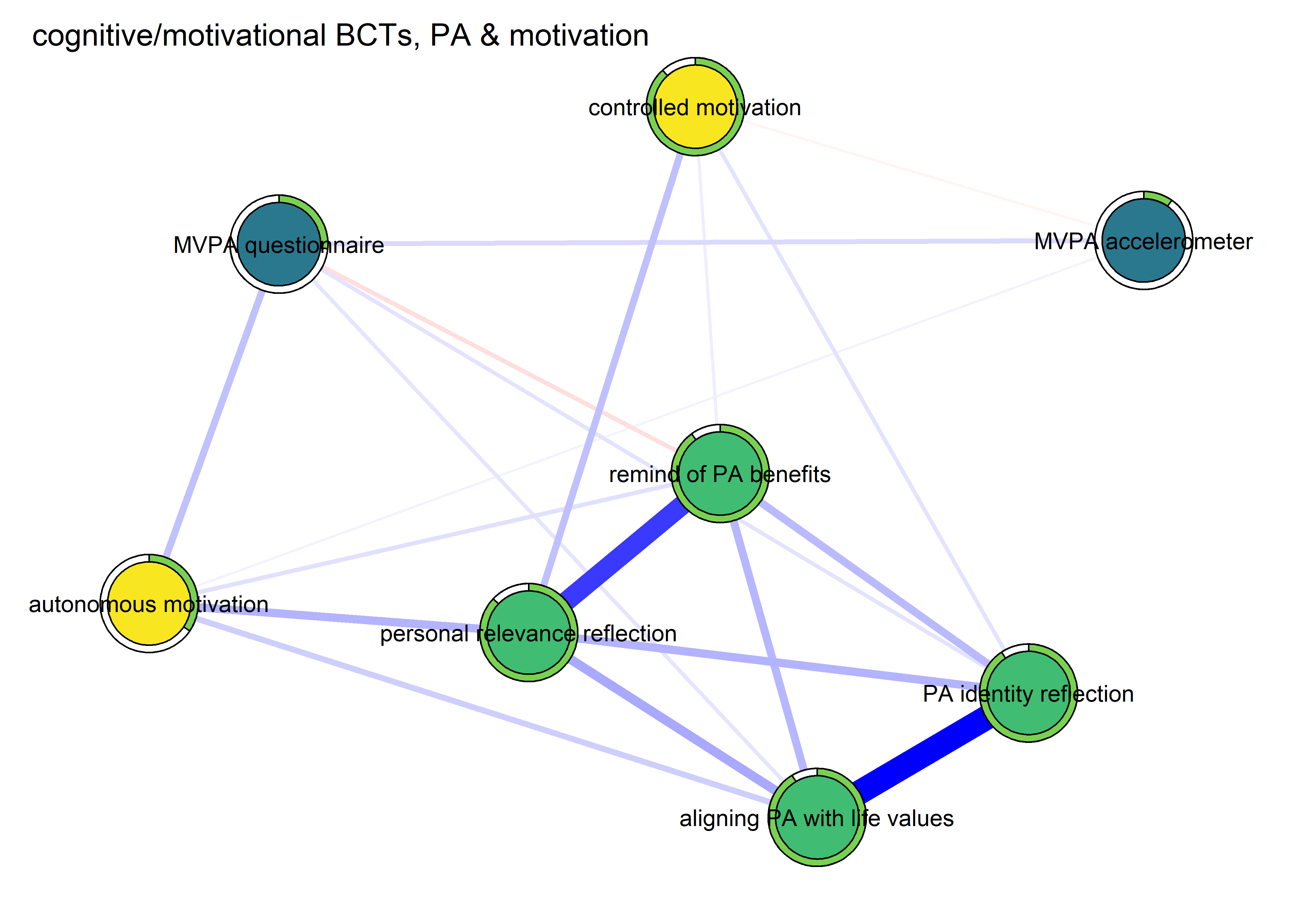
Next: Removing motivation items makes the negative connection between positive consequences and MVPA questionnaire disappear (see following plot). One explanation would be conditioning on a collider: if both physical activity and thinking about its positive consequences lead to autonomous motivation, this creates a spurious negative link between the two antecedents.
bctdf_mgm <- df %>% dplyr::select(
#  id,
#  intervention,
#  group,
#  school,
#  girl,
  'goal setting' = PA_agreementDependentBCT_01_T1,
  'own plan' = PA_agreementDependentBCT_02_T1,
  'plan by other' = PA_agreementDependentBCT_03_T1,
  'reminder of plan' = PA_agreementDependentBCT_04_T1,
  'subgoals' = PA_agreementDependentBCT_05_T1,
  'trying new PA' = PA_agreementDependentBCT_06_T1,
  'barrier identification' = PA_agreementDependentBCT_07_T1,
  'problem solving' = PA_agreementDependentBCT_08_T1,
  'PA identity reflection' = PA_agreementDependentBCT_09_T1,
  'aligning PA with life values' = PA_agreementDependentBCT_10_T1,
  'remind of PA benefits' = PA_frequencyDependentBCT_01_T1,
  'self-monitor (paper)' = PA_frequencyDependentBCT_02_T1,
  'self-monitor (app)' = PA_frequencyDependentBCT_03_T1,
#  'memory cues' = PA_frequencyDependentBCT_04_T1, # Issues with clarity of item wording
  'goal review' = PA_frequencyDependentBCT_05_T1,
  'personal relevance reflection' = PA_frequencyDependentBCT_06_T1,
  'environmental changes (home)' = PA_frequencyDependentBCT_07_T1,
  'social support' = PA_frequencyDependentBCT_08_T1,
  'analysing goal failure' = PA_frequencyDependentBCT_09_T1,
  'MVPA questionnaire' = padaysLastweek_T1,
  'MVPA accelerometer' = mvpaAccelerometer_T1,
  'intrinsic' = PA_intrinsic_T1,
  'identified' = PA_identified_T1,
  'controlled motivation' = PA_controlled_T1) %>%
 rowwise() %>%
 dplyr::transmute(
  # 'goal setting' = ifelse(`goal setting` == 1, 0, 1),
  # 'has plan' = ifelse(`own plan` == 1 & `plan by other` == 1, 0, 1),
  # 'own plan' = ifelse(`own plan` == 1, 0, 1),
  # 'plan by other' = ifelse(`plan by other` == 1, 0, 1),
  # 'reminder of plan' = ifelse(`reminder of plan` == 1, 0, 1),
  # 'subgoals' = ifelse(`subgoals` == 1, 0, 1),
  # 'trying new PA' = ifelse(`trying new PA` == 1, 0, 1),
  # 'barrier identification' = ifelse(`barrier identification` == 1, 0, 1),
  # 'problem solving' = ifelse(`problem solving` == 1, 0, 1),
  # 'barriers identified or planned for' = ifelse(`problem solving` == 1 & `barrier identification` == 1, 0, 1),
 'PA identity reflection' = ifelse(`PA identity reflection` == 1, 0, 1),
 'aligning PA with life values' = ifelse(`aligning PA with life values` == 1, 0, 1),
  # 'identity, life values' = ifelse(`PA identity reflection` == 1 & `aligning PA with life values` == 1, 0, 1),
  'remind of PA benefits' = ifelse(`remind of PA benefits` == 1, 0, 1),
  # 'monitoring PA' = ifelse(`self-monitor (paper)` == 1 & `self-monitor (app)` == 1, 0, 1),
  # 'memory cues' = ifelse(`memory cues` == 1, 0, 1),
  # 'goal review' = ifelse(`goal review` == 1, 0, 1),
  'personal relevance reflection' = ifelse(`personal relevance reflection` == 1, 0, 1),
  # 'environmental changes (home)' = ifelse(`environmental changes (home)` == 1, 0, 1),
  # 'social support' = ifelse(`social support` == 1, 0, 1),
  # 'analysing goal failure' = ifelse(`analysing goal failure` == 1, 0, 1),
  'autonomous motivation' = mean(c(identified, intrinsic), na.rm = TRUE),
#  'girl' = ifelse(girl == "girl", 1, 0),
  'controlled motivation' = ifelse(`controlled motivation` < 3, 0, 1), # If "at least partly" or more true, input 1. Normality otherwise a problem.
  'MVPA questionnaire' = `MVPA questionnaire` * 1,
  'MVPA accelerometer' = `MVPA accelerometer` * 1) %>%
  dplyr::select('MVPA questionnaire', 'MVPA accelerometer', everything()) %>%
  dplyr::select(-'autonomous motivation', -'controlled motivation')

# bctdf_mgm$`autonomous motivation`[is.nan(bctdf_mgm$`autonomous motivation`)] <- NA

labs <- names(bctdf_mgm)

bctdf_mgm <- bctdf_mgm %>% na.omit(.)
# bctdf_mgm %>% names()
mgm_variable_types <- c("g", "g", rep("c", 4))
mgm_variable_levels <- c("1", "1", rep("2", 4))
# data.frame(mgm_variable_types, mgm_variable_levels, names(bctdf_mgm))

mgm_obj <- mgm::mgm(data = bctdf_mgm,
  type = mgm_variable_types,
  level = mgm_variable_levels,
  lambdaSel = "CV",
  lambdaFolds = 10,
  pbar = FALSE,
  binarySign = TRUE)
## Note that the sign of parameter estimates is stored separately; see ?mgm

pred_obj <- predict(object = mgm_obj,
                         data = bctdf_mgm)

pred_obj$errors
# Take R2 from gaussian, CC from categorical variables
pie_errors <- c(pred_obj$errors[1, 3],
                pred_obj$errors[2, 3],
                pred_obj$errors[3:6, 4])

# Coloring nodes: make a sequence of colors from the viridis palette. We need three colors (MVPA, BCTs, motivation), and "begin" from ones that are not too dark, so that black text shows up ok.

node_colors <- c(viridis::viridis(3, begin = 0.4, end = 0.99)[1], # Color 1 for MVPA (questionnaire)
                 viridis::viridis(3, begin = 0.4, end = 0.99)[1], # Color 1 for MVPA (accelerometer)
                 rep(viridis::viridis(3, begin = 0.4, end = 0.99)[2], 4)) # 4x Color 2 for BCTs

BCT_mgm <- qgraph::qgraph(mgm_obj$pairwise$wadj,
            layout = "spring",
            repulsion = 0.99, # To nudge the network from originally bad visual state
            title = "cognitive/motivational BCTs, PA & motivation",
            edge.color = ifelse(mgm_obj$pairwise$edgecolor == "darkgreen", "blue", mgm_obj$pairwise$edgecolor),
            pie = pie_errors,
            pieColor = viridis::viridis(5, begin = 0.3, end = 0.8)[5],
            color = node_colors,
            labels = names(bctdf_mgm),
            label.cex = 0.75,
            label.scale = FALSE)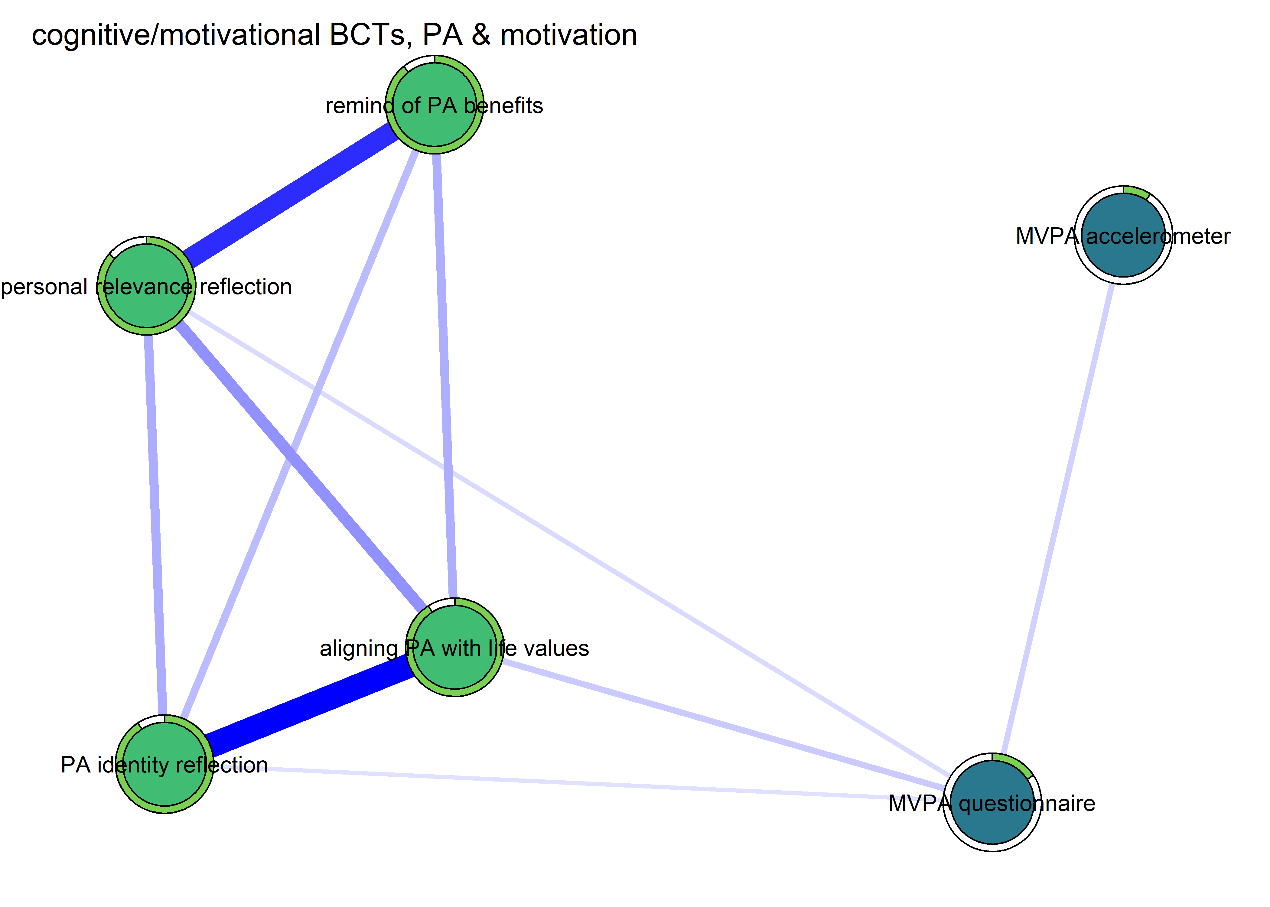
Keeping only the three items showing a presumable conditioning on a collider effect, does not lend support for the simple collider hypothesis with these variables.
bctdf_mgm <- df %>% dplyr::select(
#  id,
#  intervention,
#  group,
#  school,
#  girl,
  'goal setting' = PA_agreementDependentBCT_01_T1,
  'own plan' = PA_agreementDependentBCT_02_T1,
  'plan by other' = PA_agreementDependentBCT_03_T1,
  'reminder of plan' = PA_agreementDependentBCT_04_T1,
  'subgoals' = PA_agreementDependentBCT_05_T1,
  'trying new PA' = PA_agreementDependentBCT_06_T1,
  'barrier identification' = PA_agreementDependentBCT_07_T1,
  'problem solving' = PA_agreementDependentBCT_08_T1,
  'PA identity reflection' = PA_agreementDependentBCT_09_T1,
  'aligning PA with life values' = PA_agreementDependentBCT_10_T1,
  'remind of PA benefits' = PA_frequencyDependentBCT_01_T1,
  'self-monitor (paper)' = PA_frequencyDependentBCT_02_T1,
  'self-monitor (app)' = PA_frequencyDependentBCT_03_T1,
#  'memory cues' = PA_frequencyDependentBCT_04_T1, # Issues with clarity of item wording
  'goal review' = PA_frequencyDependentBCT_05_T1,
  'personal relevance reflection' = PA_frequencyDependentBCT_06_T1,
  'environmental changes (home)' = PA_frequencyDependentBCT_07_T1,
  'social support' = PA_frequencyDependentBCT_08_T1,
  'analysing goal failure' = PA_frequencyDependentBCT_09_T1,
  'MVPA questionnaire' = padaysLastweek_T1,
  'MVPA accelerometer' = mvpaAccelerometer_T1,
  'intrinsic' = PA_intrinsic_T1,
  'identified' = PA_identified_T1,
  'controlled motivation' = PA_controlled_T1) %>%
 rowwise() %>%
 dplyr::transmute(
  # 'goal setting' = ifelse(`goal setting` == 1, 0, 1),
  # 'has plan' = ifelse(`own plan` == 1 & `plan by other` == 1, 0, 1),
  # 'own plan' = ifelse(`own plan` == 1, 0, 1),
  # 'plan by other' = ifelse(`plan by other` == 1, 0, 1),
  # 'reminder of plan' = ifelse(`reminder of plan` == 1, 0, 1),
  # 'subgoals' = ifelse(`subgoals` == 1, 0, 1),
  # 'trying new PA' = ifelse(`trying new PA` == 1, 0, 1),
  # 'barrier identification' = ifelse(`barrier identification` == 1, 0, 1),
  # 'problem solving' = ifelse(`problem solving` == 1, 0, 1),
  # 'barriers identified or planned for' = ifelse(`problem solving` == 1 & `barrier identification` == 1, 0, 1),
 # 'PA identity reflection' = ifelse(`PA identity reflection` == 1, 0, 1),
 'aligning PA with life values' = ifelse(`aligning PA with life values` == 1, 0, 1),
  # 'identity, life values' = ifelse(`PA identity reflection` == 1 & `aligning PA with life values` == 1, 0, 1),
  'remind of PA benefits' = ifelse(`remind of PA benefits` == 1, 0, 1),
  # 'monitoring PA' = ifelse(`self-monitor (paper)` == 1 & `self-monitor (app)` == 1, 0, 1),
  # 'memory cues' = ifelse(`memory cues` == 1, 0, 1),
  # 'goal review' = ifelse(`goal review` == 1, 0, 1),
  'personal relevance reflection' = ifelse(`personal relevance reflection` == 1, 0, 1),
  # 'environmental changes (home)' = ifelse(`environmental changes (home)` == 1, 0, 1),
  # 'social support' = ifelse(`social support` == 1, 0, 1),
  # 'analysing goal failure' = ifelse(`analysing goal failure` == 1, 0, 1),
  'autonomous motivation' = mean(c(identified, intrinsic), na.rm = TRUE),
#  'girl' = ifelse(girl == "girl", 1, 0),
  'controlled motivation' = ifelse(`controlled motivation` < 3, 0, 1), # If "at least partly" or more true, input 1. Normality otherwise a problem.
  'MVPA questionnaire' = `MVPA questionnaire` * 1,
  'MVPA accelerometer' = `MVPA accelerometer` * 1) %>%
  dplyr::select('MVPA questionnaire', 'autonomous motivation', 'remind of PA benefits')

bctdf_mgm$`autonomous motivation`[is.nan(bctdf_mgm$`autonomous motivation`)] <- NA

labs <- names(bctdf_mgm)

bctdf_mgm <- bctdf_mgm %>% na.omit(.)
# bctdf_mgm %>% names()
mgm_variable_types <- c("g", "g", "c")
mgm_variable_levels <- c("1", "1", "2")
# data.frame(mgm_variable_types, mgm_variable_levels, names(bctdf_mgm))

mgm_obj <- mgm::mgm(data = bctdf_mgm,
  type = mgm_variable_types,
  level = mgm_variable_levels,
  lambdaSel = "CV",
  lambdaFolds = 10,
  pbar = FALSE,
  binarySign = TRUE)
## Note that the sign of parameter estimates is stored separately; see ?mgm

pred_obj <- predict(object = mgm_obj,
                         data = bctdf_mgm)

pred_obj$errors
# Take R2 from gaussian, CC from categorical variables
pie_errors <- c(pred_obj$errors[1, 3],
                pred_obj$errors[2, 3],
                pred_obj$errors[3, 4])

# Coloring nodes: make a sequence of colors from the viridis palette. We need three colors (MVPA, BCTs, motivation), and "begin" from ones that are not too dark, so that black text shows up ok.

node_colors <- c(viridis::viridis(3, begin = 0.4, end = 0.99)[1], # Color 1 for MVPA (questionnaire)
                 viridis::viridis(3, begin = 0.4, end = 0.99)[3], # Color 3 for motivation (autonomous)
                 viridis::viridis(3, begin = 0.4, end = 0.99)[2]) # Color 2 for BCTs

BCT_mgm <- qgraph::qgraph(mgm_obj$pairwise$wadj,
            layout = "spring",
            repulsion = 0.99, # To nudge the network from originally bad visual state
            title = "cognitive/motivational BCTs, PA & motivation",
            edge.color = ifelse(mgm_obj$pairwise$edgecolor == "darkgreen", "blue", mgm_obj$pairwise$edgecolor),
            pie = pie_errors,
            pieColor = viridis::viridis(5, begin = 0.3, end = 0.8)[5],
            color = node_colors,
            labels = names(bctdf_mgm),
            label.cex = 0.75,
            label.scale = FALSE)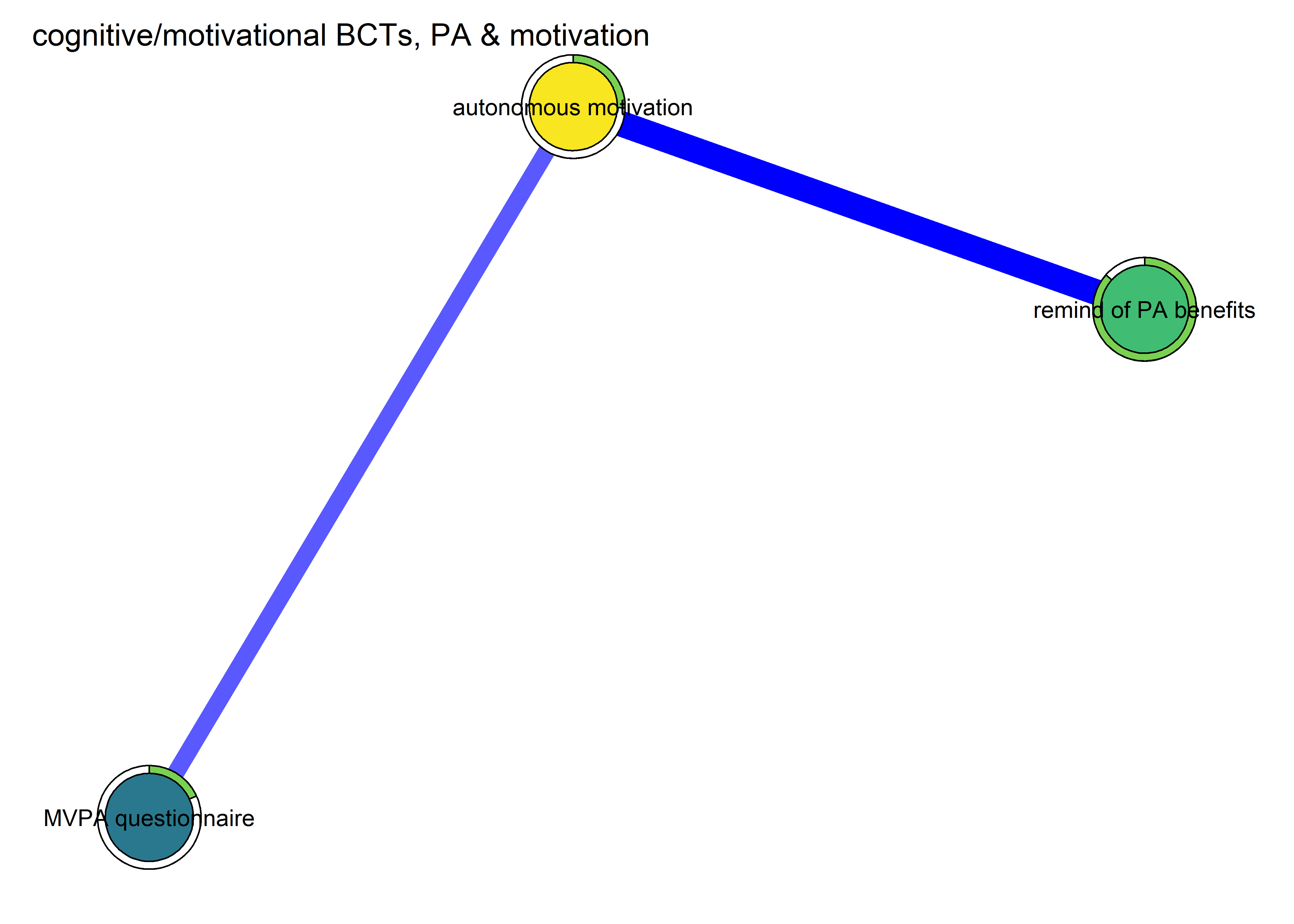
Environmental variables (group, opportunities)
Environmental opportunities include having enough money to be physically active, biking and hiking tracks in one’s environment, needed PA equipment (gear), facilities for being physically active (such as sports halls/centres, gyms) nearby, not feeling like lack of PA gear is an obstackle for being active, not being too busy with school, hobbies and/or friends, having good opportunities to be active at home, and not feeling like one’s family or religion restricts their activity.
environmentdf_mgm_T1 <- df %>%
  dplyr::select('group feels safe' = groupFeelsSafe_T1,
  'group listens to me' = groupListensToMe_T1,
  'group supports me' = groupSupportsMe_T1,
  'group understands me' = groupUnderstandsMe_T1,
  'group values me' = groupValuesMe_T1,
  "enough money" = PA_opportunities_01_T1,
  "biking and hiking tracks" = PA_opportunities_02_T1,
  "has PA gear" = PA_opportunitiesReverseCoded_03_T1,
  "facilities (e.g. gyms)" = PA_opportunities_04_T1,
  "PA gear no obstacle" = PA_opportunities_05_T1,
  "life not too busy" = PA_opportunitiesReverseCoded_06_T1,
  "opportunities at home" = PA_opportunities_07_T1,
  "religion or family" = PA_opportunitiesReverseCoded_08_T1,
  'MVPA survey' = padaysLastweek_T1,
  'MVPA accelerometer' = mvpaAccelerometer_T1) %>%
 rowwise() %>%
 mutate("religion or family" = ifelse(`religion or family` < 7, 0, 1)) %>% # highly skewed, so dichotomised
  dplyr::select('MVPA survey', 'MVPA accelerometer', everything())

labs <- names(environmentdf_mgm_T1)

# mgm wants full data, see package missForest for imputation methods
environmentdf_mgm_T1 <- environmentdf_mgm_T1 %>% na.omit(.)
# environmentdf_mgm %>% names()
mgm_variable_types <- c(rep("g", 14), rep("c", 1))
mgm_variable_levels <- c(rep("1", 14), rep("2", 1))
# data.frame(mgm_variable_types, mgm_variable_levels, names(environmentdf_mgm))

mgm_obj_T1 <- mgm::mgm(data = environmentdf_mgm_T1,
  type = mgm_variable_types,
  level = mgm_variable_levels,
  lambdaSel = "EBIC",
  # lambdaFolds = 10,
  pbar = FALSE,
  binarySign = TRUE)
## Note that the sign of parameter estimates is stored separately; see ?mgm

# Node pies:
# pies_T1 <- environmentdf_mgm_T1 %>%
#   dplyr::summarise_all(~mean(., na.rm = TRUE)) # results in a series of means, which is ok for dichotomous vars
# pies_T1[1] <- pies_T1[1] / 7
# pies_T1[2] <- pies_T1[2] / max(environmentdf_mgm_T1$`MVPA accelerometer`, na.rm = TRUE)
# pies_T1[20] <- pies_T1[20] / 5


node_colors <- c(viridis::viridis(3, begin = 0.4, end = 0.99)[1], # Color 1 for MVPA (questionnaire)
                 viridis::viridis(3, begin = 0.4, end = 0.99)[1], # Color 1 for MVPA (accelerometer)
                 rep(viridis::viridis(3, begin = 0.4, end = 0.99)[2], 5), # 5x Color 2 for group-variables
                 rep(viridis::viridis(3, begin = 0.4, end = 0.99)[3], 8)) # Color 3 for opportunities

# environment_mgm_T1 <- qgraph::qgraph(mgm_obj_T1$pairwise$wadj,
#             layout = "spring",
#             repulsion = 0.99, # To nudge the network from originally bad visual state
#             edge.color = ifelse(mgm_obj_T1$pairwise$edgecolor == "darkgreen", "blue", mgm_obj_T1$pairwise$edgecolor),
#             # pie = pies_T1,
#             # pieColor = pie_colors_T1,
#             pieColor = node_colors,
#             labels = names(environmentdf_mgm_T1),
#             # pieBorder = 1,
#             label.cex = 0.75,
#             cut = 0,
#             edge.labels = TRUE,
#             label.scale = FALSE)

environment_mgm_T1_circle <- qgraph::qgraph(mgm_obj_T1$pairwise$wadj,
            layout = "circle",
            title = "Mixed graphical model: PA, group environment & opportunities",
            edge.color = ifelse(mgm_obj_T1$pairwise$edgecolor == "darkgreen", "blue", mgm_obj_T1$pairwise$edgecolor),
            # pie = pies_T1,
            # pieColor = viridis::viridis(5, begin = 0.3, end = 0.8)[5],
            color = node_colors,
            labels = names(environmentdf_mgm_T1),
            label.cex = 0.75,
            cut = 0,
            label.scale = FALSE)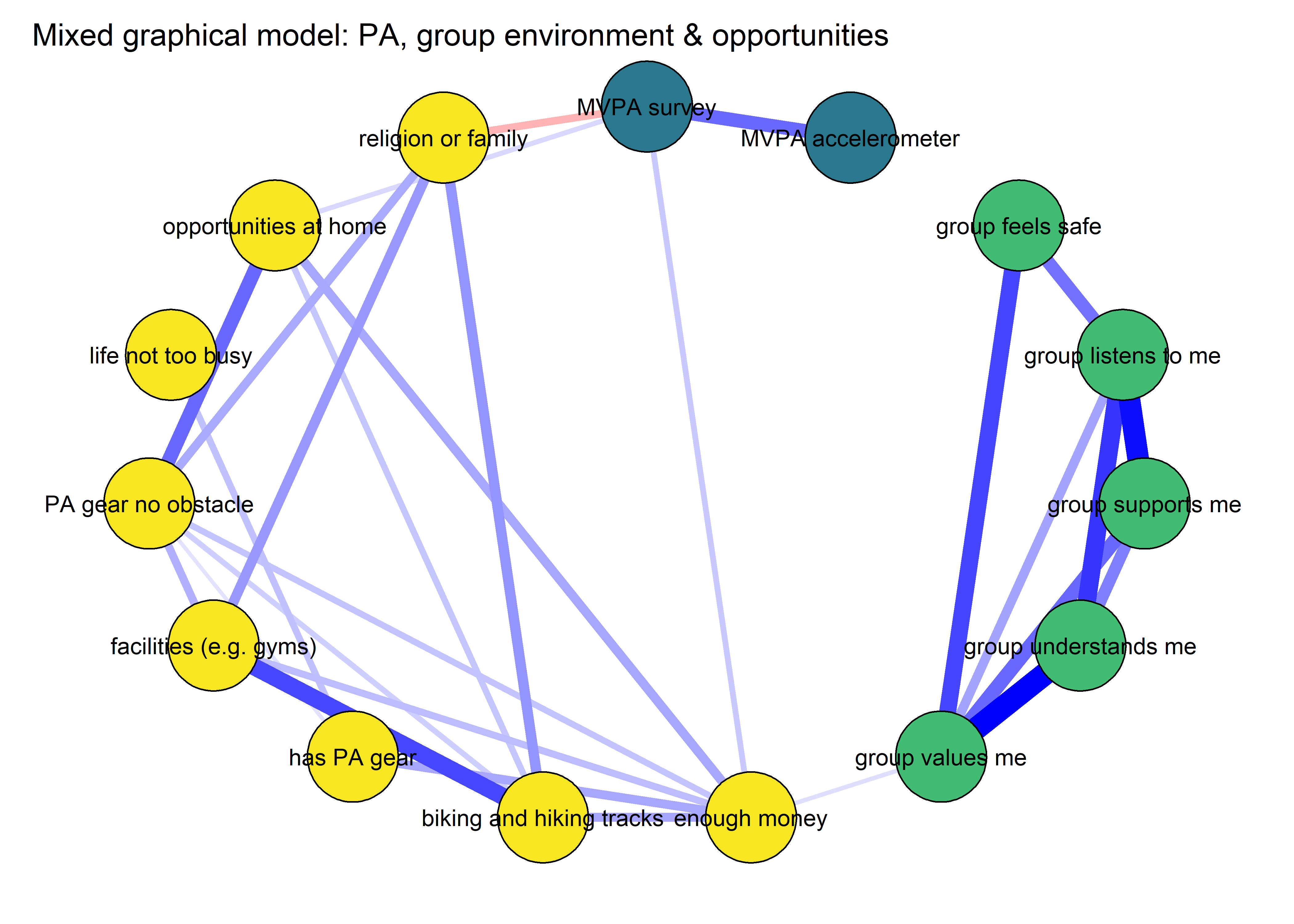
Exercise types
The first network is an Ising model with all participants.
exerciseTypes_df <- lmi %>% select(Kys0051.1:Kys0064.1) %>%
  dplyr::select(contains(".1")) %>%
  dplyr::mutate_all(funs(replace_na(., 0)))
# exerciseTypes_df$track <- df$track
# exerciseTypes_df$girl <- df$girl

names(exerciseTypes_df) <- c("Team ball games",
                             "Other ball games",
                             "Gym training",
                             "Combat sports",
                             "Fitness classes",
                             "Home workout",
                             "Cycling",
                             "Swimming",
                             "Walking",
                             "Running",
                             "Skiing",
                             "Roller skating",
                             "Horseback riding",
                             "Other"
                             )

exerciseTypes_df %>% dplyr::summarise_all(funs(sum))
# Roller skating has only 8 observations; leave out
exerciseTypes_df <- exerciseTypes_df %>% dplyr::select(-`Roller skating`)

# Variable types are muddled, change all to numeric
exerciseTypes_df <- as.data.frame(purrr::map(exerciseTypes_df, `class<-`, c("numeric")))

# Change data frame to type tbl to allow for spaces
exerciseTypes_df <- as.tbl(exerciseTypes_df)

# Take all names, replace the dots with space
names(exerciseTypes_df) <- stringr::str_replace_all(names(exerciseTypes_df), pattern = "\\.", replacement = " ")

exerciseTypes_network <- bootnet::estimateNetwork(exerciseTypes_df, default="IsingFit")
##
  |
  |                                                                 |   0%
  |
  |=====                                                            |   8%
  |
  |==========                                                       |  15%
  |
  |===============                                                  |  23%
  |
  |====================                                             |  31%
  |
  |=========================                                        |  38%
  |
  |==============================                                   |  46%
  |
  |===================================                              |  54%
  |
  |========================================                         |  62%
  |
  |=============================================                    |  69%
  |
  |==================================================               |  77%
  |
  |=======================================================          |  85%
  |
  |============================================================     |  92%
  |
  |=================================================================| 100%

# Create means for filling nodes
piefill <- exerciseTypes_df %>%
  summarise_all(funs(mean(., na.rm = TRUE)))

# Plot network
exerciseTypes_ising <- plot(
  exerciseTypes_network,
  layout = "spring",
  label.scale = FALSE,
  title = "Ising fit: self-reported exercise types",
  # label.cex = 0.75,
  pie = piefill,
  color = "skyblue",
  pieBorder = 1)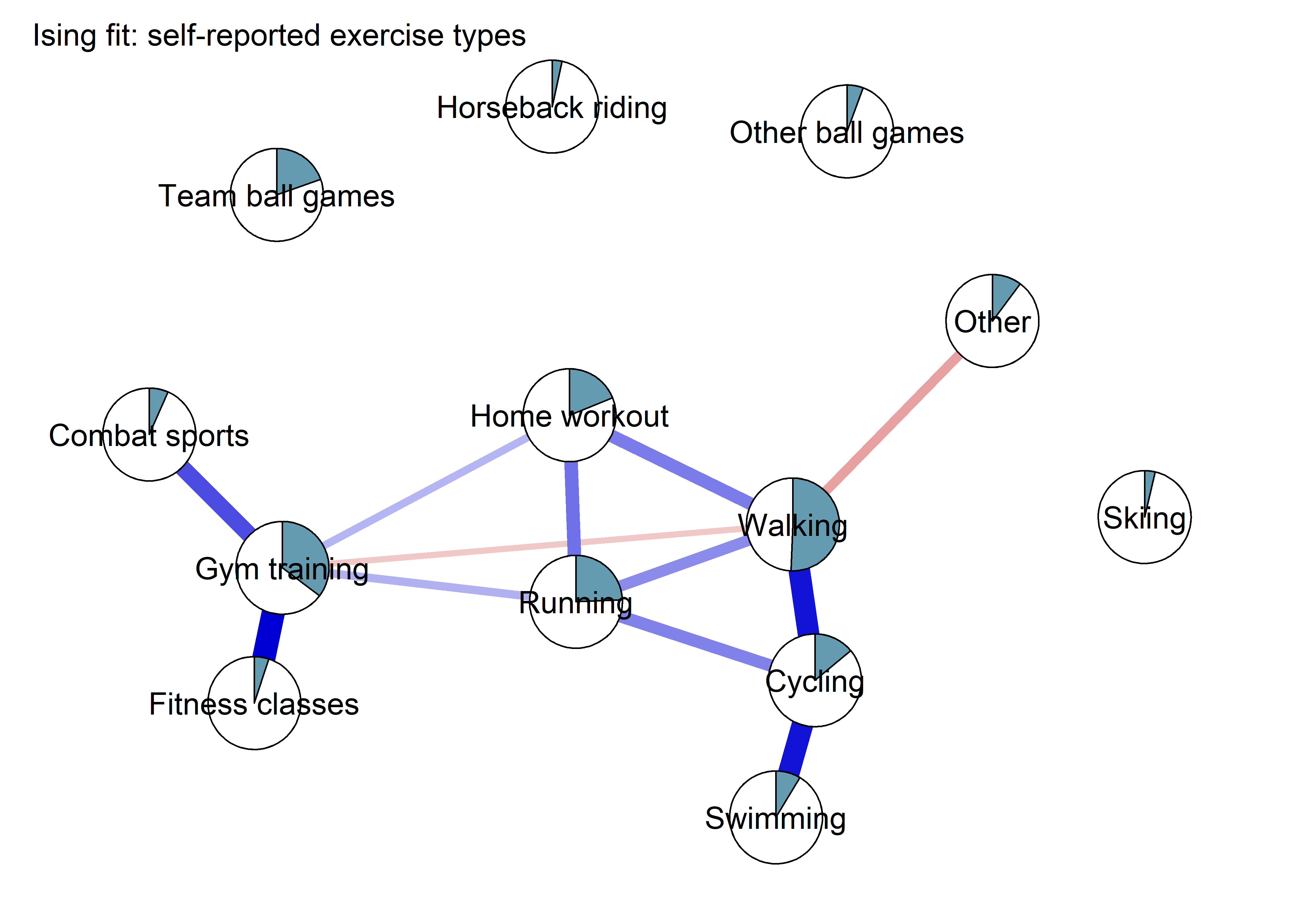
Same network, but estimated with mgm:
exerciseTypes_df <- lmi %>% select(Kys0051.1:Kys0064.1) %>%
  dplyr::select(contains(".1")) %>%
  dplyr::mutate_all(funs(replace_na(., 0)))
# exerciseTypes_df$track <- df$track
# exerciseTypes_df$girl <- df$girl
# exerciseTypes_df$`PA accelerometer` <- df$mvpaAccelerometer_T1
# exerciseTypes_df$`PA self-report` <- df$padaysLastweek_T1

names(exerciseTypes_df) <- c("Team ball games",
                             "Other ball games",
                             "Gym training",
                             "Combat sports",
                             "Fitness classes",
                             "Home workout",
                             "Cycling",
                             "Swimming",
                             "Walking",
                             "Running",
                             "Skiing",
                             "Roller skating",
                             "Horseback riding",
                             "Other"
                             # "PA accelerometer",
                             # "PA self-report"
                             )

# Roller skating has only 8 observations; leave out
exerciseTypes_df <- exerciseTypes_df %>% dplyr::select(-`Roller skating`)

# Variable types are muddled, change all to numeric
exerciseTypes_df <- as.data.frame(purrr::map(exerciseTypes_df, `class<-`, c("numeric")))

# Change data frame to type tbl to allow for spaces
exerciseTypes_df <- as.tbl(exerciseTypes_df)

# Take all names, replace the dots with space
names(exerciseTypes_df) <- stringr::str_replace_all(names(exerciseTypes_df), pattern = "\\.", replacement = " ")

# Remove incomplete cases
exerciseTypes_df_fullobs <- exerciseTypes_df %>% na.omit()

# Tell mgm, that the first 14 variables are categorical and the last two are gaussian
exerciseTypes_df_variable_types <- c(rep("c", 13))
exerciseTypes_df_variable_levels <- c(rep("2", 13))
# data.frame(exerciseTypes_df_variable_types, exerciseTypes_df_variable_levels, names(exerciseTypes_df))

mgm_obj <- mgm::mgm(data = exerciseTypes_df_fullobs,
  type = exerciseTypes_df_variable_types,
  level = exerciseTypes_df_variable_levels,
  lambdaSel = "CV",
  lambdaFolds = 10,
  pbar = FALSE,
  binarySign = TRUE)
## Note that the sign of parameter estimates is stored separately; see ?mgm

pred_obj <- predict(object = mgm_obj,
                         data = exerciseTypes_df_fullobs)

# pred_obj$errors

# Take R2 from gaussian, CC from categorical variables
pie_errors <- c(pred_obj$errors[1:13, 4])

# Define node colors
node_colors <- c(rep(viridis::viridis(3, begin = 0.4, end = 0.95)[1], 13))

exerciseTypes_mgm <- qgraph::qgraph(mgm_obj$pairwise$wadj,
            layout = "spring",
            repulsion = 0.999, # To nudge the network from originally bad visual state
            title = "Mixed graphical model: Types of reported physical activity",
            edge.color = ifelse(mgm_obj$pairwise$edgecolor == "darkgreen", "blue", mgm_obj$pairwise$edgecolor),
            pie = pie_errors,
            pieColor = viridis::viridis(3, begin = 0.4, end = 0.95)[2],
            color = node_colors,
            labels = names(exerciseTypes_df_fullobs),
            label.cex = 0.75,
            label.scale = FALSE,
            label.color = c(rep("black", 13)))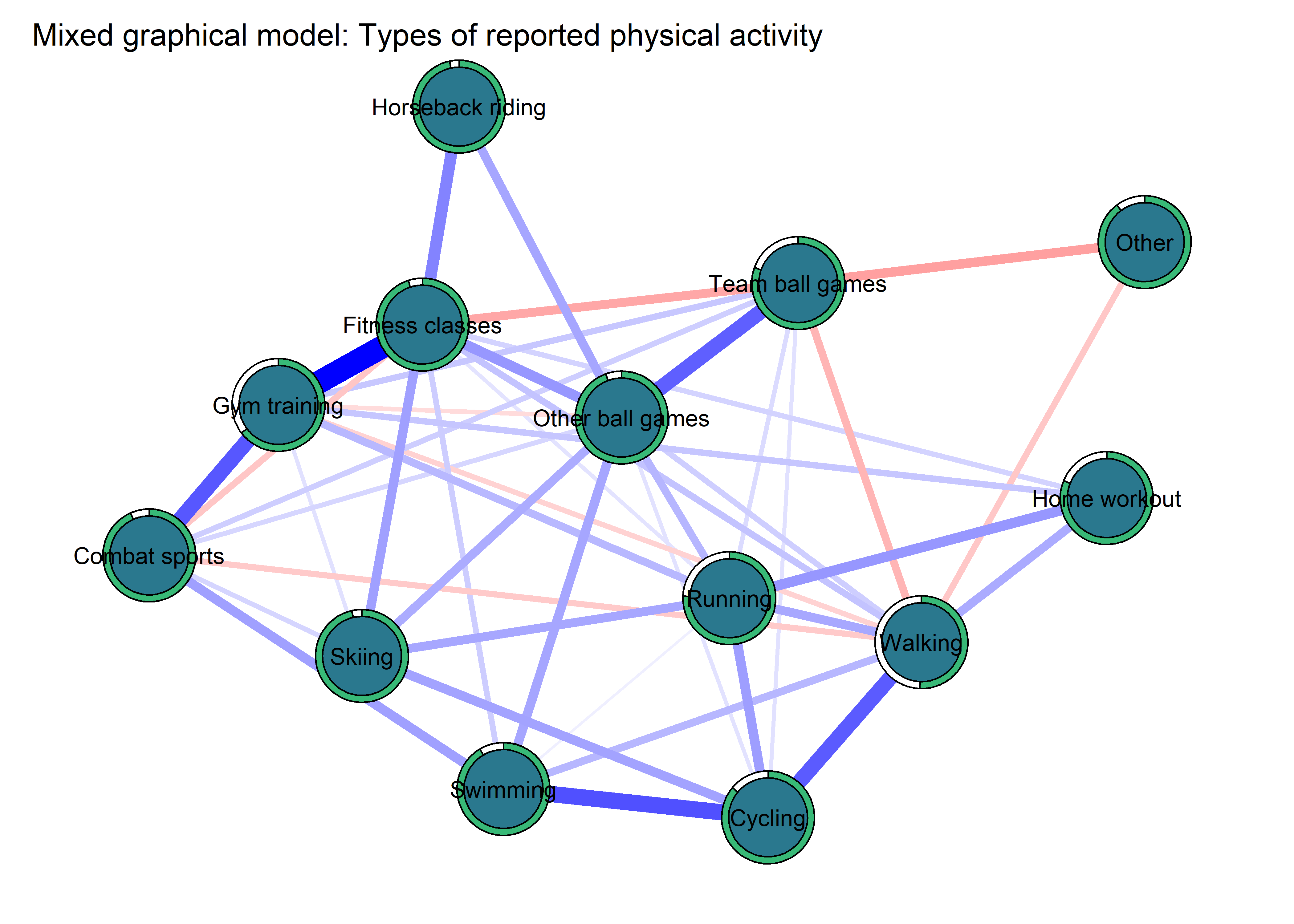
Below, we average the layout and plot these networks side-by-side for comparison.
avglayout <- qgraph::averageLayout(exerciseTypes_mgm, exerciseTypes_ising)

layout(t(1:2))

exerciseTypes_ising <- plot(
  exerciseTypes_network,
  layout = avglayout,
  label.scale = FALSE,
  title = "Ising fit (EBIC model selection)",
  label.cex = 0.75,
  pie = piefill,
  color = "skyblue",
  pieBorder = 1)

exerciseTypes_mgm <- qgraph::qgraph(mgm_obj$pairwise$wadj,
            layout = avglayout,
            repulsion = 0.999, # To nudge the network from originally bad visual state
            title = "Mixed graphical model (Cross-validation)",
            edge.color = ifelse(mgm_obj$pairwise$edgecolor == "darkgreen", "blue", mgm_obj$pairwise$edgecolor),
            pie = pie_errors,
            pieColor = viridis::viridis(3, begin = 0.4, end = 0.95)[2],
            color = node_colors,
            labels = names(exerciseTypes_df_fullobs),
            label.cex = 0.75,
            label.scale = FALSE,
            label.color = c(rep("black", 13))
            )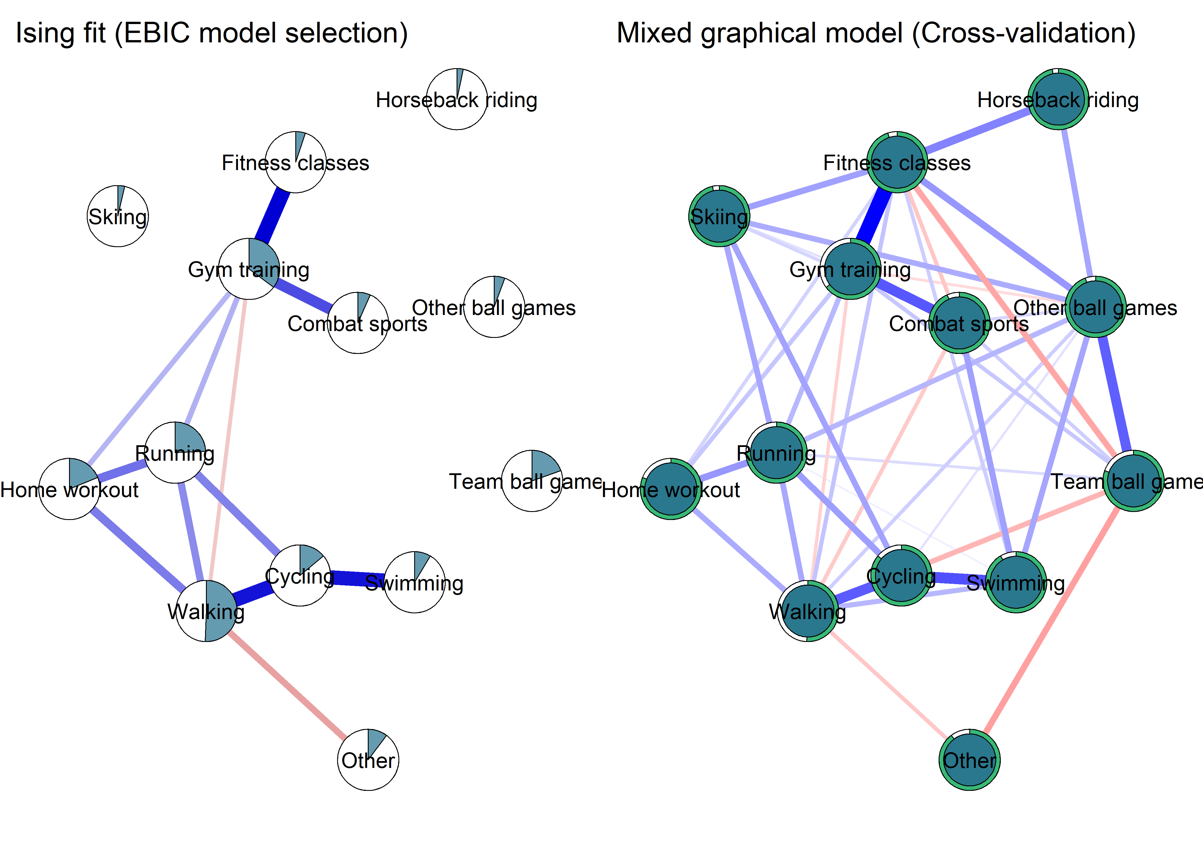
Graph below includes the moderate-to-vigorous physical activity measures, and shows a mixed graphical model with model selection done by cross-validation.
exerciseTypes_df <- lmi %>% select(Kys0051.1:Kys0064.1) %>%
  dplyr::select(contains(".1")) %>%
  dplyr::mutate_all(funs(replace_na(., 0)))
# exerciseTypes_df$track <- df$track
# exerciseTypes_df$girl <- df$girl
exerciseTypes_df$`PA accelerometer` <- df$mvpaAccelerometer_T1
exerciseTypes_df$`PA self-report` <- df$padaysLastweek_T1

names(exerciseTypes_df) <- c("Team ball games",
                             "Other ball games",
                             "Gym training",
                             "Combat sports",
                             "Fitness classes",
                             "Home workout",
                             "Cycling",
                             "Swimming",
                             "Walking",
                             "Running",
                             "Skiing",
                             "Roller skating",
                             "Horseback riding",
                             "Other",
                             "PA accelerometer",
                             "PA self-report"
                             )

# Roller skating has only 8 observations; leave out
exerciseTypes_df <- exerciseTypes_df %>% dplyr::select(-`Roller skating`)

# Variable types are muddled, change all to numeric
exerciseTypes_df <- as.data.frame(purrr::map(exerciseTypes_df, `class<-`, c("numeric")))

# Change data frame to type tbl to allow for spaces
exerciseTypes_df <- as.tbl(exerciseTypes_df)

# Take all names, replace the dots with space
names(exerciseTypes_df) <- stringr::str_replace_all(names(exerciseTypes_df), pattern = "\\.", replacement = " ")

# Remove incomplete cases
exerciseTypes_df_fullobs <- exerciseTypes_df %>% na.omit()

# Tell mgm, that the first 14 variables are categorical and the last two are gaussian
exerciseTypes_df_variable_types <- c(rep("c", 13), rep("g", 2))
exerciseTypes_df_variable_levels <- c(rep("2", 13), rep("1", 2))
# data.frame(exerciseTypes_df_variable_types, exerciseTypes_df_variable_levels, names(exerciseTypes_df))

mgm_obj_CV <- mgm::mgm(data = exerciseTypes_df_fullobs,
  type = exerciseTypes_df_variable_types,
  level = exerciseTypes_df_variable_levels,
  lambdaSel = "CV",
  lambdaFolds = 10,
  pbar = FALSE,
  binarySign = TRUE)
## Note that the sign of parameter estimates is stored separately; see ?mgm

pred_obj <- predict(object = mgm_obj_CV,
                         data = exerciseTypes_df_fullobs)

# pred_obj$errors

# Take R2 from gaussian, CC from categorical variables
pie_errors <- c(pred_obj$errors[1:13, 4],
                pred_obj$errors[14:15, 3])

# Define node colors
node_colors <- c(rep(viridis::viridis(3, begin = 0.4, end = 0.95)[1], 13),
                 rep(viridis::viridis(3, begin = 0.4, end = 0.95)[3], 2))

exerciseTypes_mgm_withMeasures <- qgraph::qgraph(mgm_obj_CV$pairwise$wadj,
            layout = "spring",
            repulsion = 0.99, # To nudge the network from originally bad visual state
            title = "Mixed graphical model: Types of reported physical activity and their relations to measured MVPA",
            edge.color = ifelse(mgm_obj_CV$pairwise$edgecolor == "darkgreen", "blue", mgm_obj_CV$pairwise$edgecolor),
            pie = pie_errors,
            pieColor = viridis::viridis(3, begin = 0.4, end = 0.95)[2],
            color = node_colors,
            labels = names(exerciseTypes_df_fullobs),
            label.cex = 0.75,
            label.scale = FALSE,
            label.color = c(rep("black", 15)))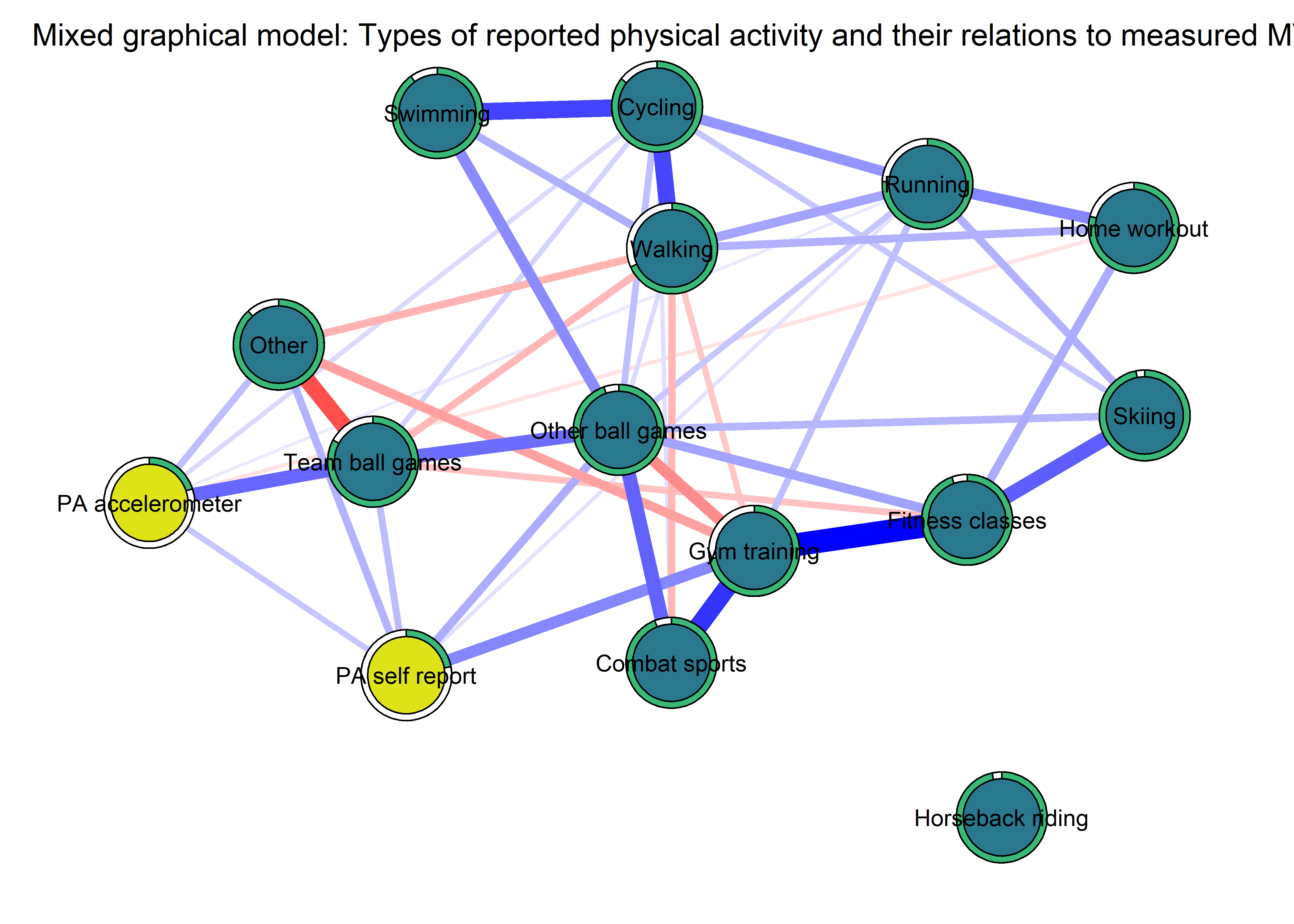
The next graph is identical, except that model selection is done by the Extended Bayesian Information Criterion (EBIC).
exerciseTypes_df <- lmi %>% select(Kys0051.1:Kys0064.1) %>%
  dplyr::select(contains(".1")) %>%
  dplyr::mutate_all(funs(replace_na(., 0)))
# exerciseTypes_df$track <- df$track
# exerciseTypes_df$girl <- df$girl
exerciseTypes_df$`PA accelerometer` <- df$mvpaAccelerometer_T1
exerciseTypes_df$`PA self-report` <- df$padaysLastweek_T1

names(exerciseTypes_df) <- c("Team ball games",
                             "Other ball games",
                             "Gym training",
                             "Combat sports",
                             "Fitness classes",
                             "Home workout",
                             "Cycling",
                             "Swimming",
                             "Walking",
                             "Running",
                             "Skiing",
                             "Roller skating",
                             "Horseback riding",
                             "Other",
                             "PA accelerometer",
                             "PA self-report"
                             )

# Roller skating has only 8 observations; leave out
exerciseTypes_df <- exerciseTypes_df %>% dplyr::select(-`Roller skating`)

# Variable types are muddled, change all to numeric
exerciseTypes_df <- as.data.frame(purrr::map(exerciseTypes_df, `class<-`, c("numeric")))

# Change data frame to type tbl to allow for spaces
exerciseTypes_df <- as.tbl(exerciseTypes_df)

# Take all names, replace the dots with space
names(exerciseTypes_df) <- stringr::str_replace_all(names(exerciseTypes_df), pattern = "\\.", replacement = " ")

# Remove incomplete cases
exerciseTypes_df_fullobs <- exerciseTypes_df %>% na.omit()

# Tell mgm, that the first 14 variables are categorical and the last two are gaussian
exerciseTypes_df_variable_types <- c(rep("c", 13), rep("g", 2))
exerciseTypes_df_variable_levels <- c(rep("2", 13), rep("1", 2))
# data.frame(exerciseTypes_df_variable_types, exerciseTypes_df_variable_levels, names(exerciseTypes_df))

mgm_obj_EBIC <- mgm::mgm(data = exerciseTypes_df_fullobs,
  type = exerciseTypes_df_variable_types,
  level = exerciseTypes_df_variable_levels,
  lambdaSel = "EBIC",
  # lambdaFolds = 10,
  pbar = FALSE,
  binarySign = TRUE)
## Note that the sign of parameter estimates is stored separately; see ?mgm

pred_obj2 <- predict(object = mgm_obj_EBIC,
                         data = exerciseTypes_df_fullobs)

# pred_obj$errors

# Take R2 from gaussian, CC from categorical variables
pie_errors2 <- c(pred_obj2$errors[1:13, 4],
                pred_obj2$errors[14:15, 3])

# Define node colors
node_colors <- c(rep(viridis::viridis(3, begin = 0.4, end = 0.95)[1], 13),
                 rep(viridis::viridis(3, begin = 0.4, end = 0.95)[3], 2))

exerciseTypes_mgm_withMeasures2 <- qgraph::qgraph(mgm_obj_EBIC$pairwise$wadj,
            layout = "spring",
            repulsion = 0.99, # To nudge the network from originally bad visual state
            title = "Mixed graphical model: Types of reported physical activity and their relations to measured MVPA",
            edge.color = ifelse(mgm_obj_EBIC$pairwise$edgecolor == "darkgreen", "blue",
                                mgm_obj_EBIC$pairwise$edgecolor),
            pie = pie_errors2,
            pieColor = viridis::viridis(3, begin = 0.4, end = 0.95)[2],
            color = node_colors,
            labels = names(exerciseTypes_df_fullobs),
            label.cex = 0.75,
            label.scale = FALSE,
            label.color = c(rep("black", 15)))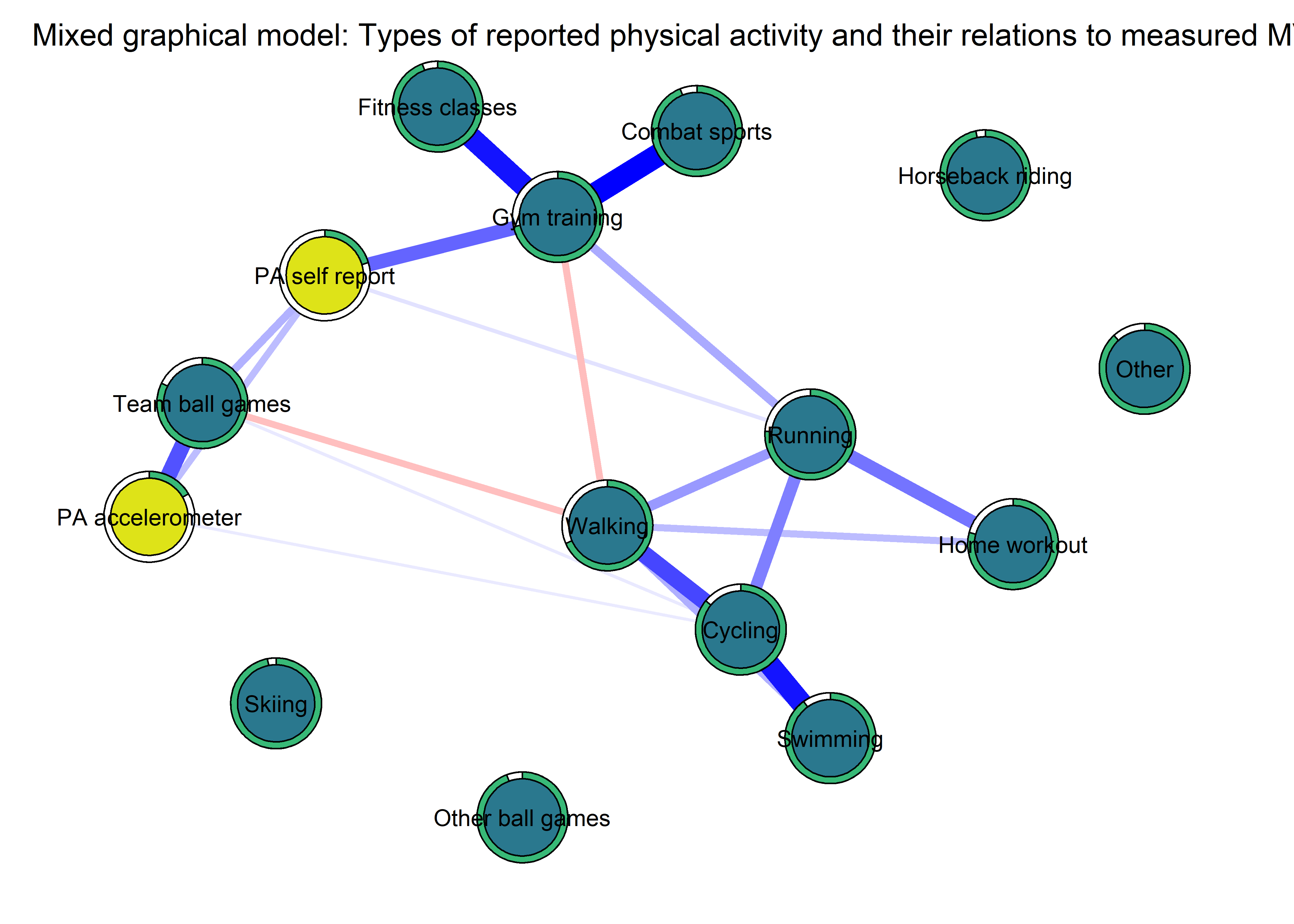
# exerciseTypes_mgm_withMeasures_cor <- qgraph::qgraph(qgraph::cor_auto(exerciseTypes_df),
#             layout = "spring",
#             repulsion = 0.99, # To nudge the network from originally bad visual state
#             title = "Bivariate correlations",
#             pie = pie_errors2,
#             pieColor = viridis::viridis(3, begin = 0.4, end = 0.95)[2],
#             color = node_colors,
#             edge.labels = TRUE,
#             labels = names(exerciseTypes_df),
#             label.cex = 0.75,
#             label.scale = FALSE)
To compare the two previous graphs, we again average the layout and plot them next to each other.
avglayout <- qgraph::averageLayout(exerciseTypes_mgm_withMeasures, exerciseTypes_mgm_withMeasures2)

layout(t(1:2))

qgraph::qgraph(mgm_obj_CV$pairwise$wadj,
            layout = avglayout,
            title = "Mixed graphical model (Cross-validation)",
            edge.color = ifelse(mgm_obj_CV$pairwise$edgecolor == "darkgreen", "blue", mgm_obj_CV$pairwise$edgecolor),
            pie = pie_errors2,
            pieColor = viridis::viridis(3, begin = 0.4, end = 0.95)[2],
            color = node_colors,
            labels = names(exerciseTypes_df_fullobs),
            label.cex = 0.75,
            label.scale = FALSE,
            label.color = c(rep("black", 13)))

qgraph::qgraph(mgm_obj_EBIC$pairwise$wadj,
            layout = avglayout,
            title = "Mixed graphical model (EBIC model selection)",
            edge.color = ifelse(mgm_obj_EBIC$pairwise$edgecolor == "darkgreen", "blue", mgm_obj_EBIC$pairwise$edgecolor),
            pie = pie_errors2,
            pieColor = viridis::viridis(3, begin = 0.4, end = 0.95)[2],
            color = node_colors,
            labels = names(exerciseTypes_df_fullobs),
            label.cex = 0.75,
            label.scale = FALSE,
            label.color = c(rep("black", 15)))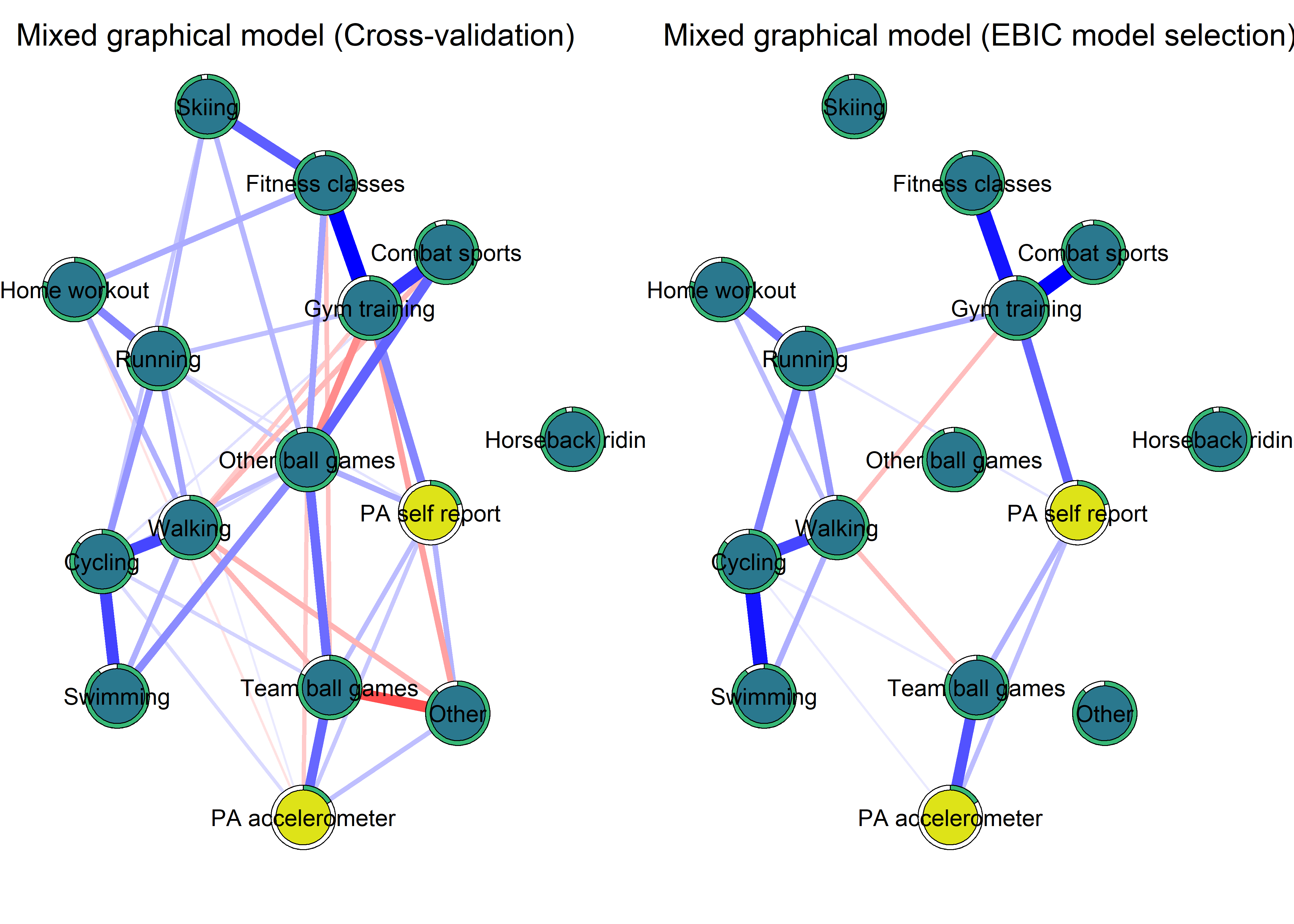
Bivariate correlations
Table below shows, how correlations between exercise types differ between the accelerometer and self-reported MVPA measure.
exerciseTypes_df <- lmi %>% select(Kys0051.1:Kys0064.1) %>%
  dplyr::select(contains(".1")) %>%
  dplyr::mutate_all(funs(replace_na(., 0)))
# exerciseTypes_df$track <- df$track
# exerciseTypes_df$girl <- df$girl
exerciseTypes_df$`PA accelerometer` <- df$mvpaAccelerometer_T1
exerciseTypes_df$`PA self-report` <- df$padaysLastweek_T1

names(exerciseTypes_df) <- c("Team ball games",
                             "Other ball games",
                             "Gym training",
                             "Combat sports",
                             "Fitness classes",
                             "Home workout",
                             "Cycling",
                             "Swimming",
                             "Walking",
                             "Running",
                             "Skiing",
                             "Roller skating",
                             "Horseback riding",
                             "Other",
                             "PA accelerometer",
                             "PA self-report"
                             )

# Roller skating has only 8 observations; leave out
exerciseTypes_df <- exerciseTypes_df %>% dplyr::select(-`Roller skating`)

# Variable types are muddled, change all to numeric
exerciseTypes_df <- as.data.frame(purrr::map(exerciseTypes_df, `class<-`, c("numeric")))

# Change data frame to type tbl to allow for spaces
exerciseTypes_df <- as.tbl(exerciseTypes_df)

# Take all names, replace the dots with space
names(exerciseTypes_df) <- stringr::str_replace_all(names(exerciseTypes_df), pattern = "\\.", replacement = " ")

qgraph::cor_auto(exerciseTypes_df) %>% data.frame() %>%
  dplyr::mutate(variable = names(exerciseTypes_df)) %>%
  dplyr::mutate_at(vars(PA.accelerometer, PA.self.report), funs(round(., 3))) %>%
  dplyr::select(variable, PA.accelerometer, PA.self.report) %>%
  dplyr::mutate(diff = PA.accelerometer - PA.self.report) %>%
  dplyr::arrange(desc(abs(diff))) %>%
  dplyr::filter(variable != "PA accelerometer", variable != "PA self report") %>%
  DT::datatable(caption = "Bivariate correlations between PA measures and self-reported activity types")
Chunked BCTs, PA, motivation
This section shows the correlations structure between BCTs (lumped into chunks based on whether they relate to frequency or agreement), motivational regulations and MVPA (self-reported MVPA the previous week and accelerometer-measured MVPA the following week).
Note: This is only to demonstrate data exploration, as many assumptions (such as multivariate normality, homogeneity, multilevel structure) are not accounted for.
bivariate_BCTs <- df %>% dplyr::select(
  'goal setting' = PA_agreementDependentBCT_01_T1,
  'own plan' = PA_agreementDependentBCT_02_T1,
  'plan by other' = PA_agreementDependentBCT_03_T1,
  'reminder of plan' = PA_agreementDependentBCT_04_T1,
  'subgoals' = PA_agreementDependentBCT_05_T1,
  'trying new PA' = PA_agreementDependentBCT_06_T1,
  'barrier identification' = PA_agreementDependentBCT_07_T1,
  'problem solving' = PA_agreementDependentBCT_08_T1,
  'PA identity reflection' = PA_agreementDependentBCT_09_T1,
  'aligning PA with life values' = PA_agreementDependentBCT_10_T1,
  'remind of PA benefits' = PA_frequencyDependentBCT_01_T1,
  'self-monitor (paper)' = PA_frequencyDependentBCT_02_T1,
  'self-monitor (app)' = PA_frequencyDependentBCT_03_T1,
  'memory cues' = PA_frequencyDependentBCT_04_T1,
  'goal review' = PA_frequencyDependentBCT_05_T1,
  'personal relevance reflection' = PA_frequencyDependentBCT_06_T1,
  'environmental changes (home)' = PA_frequencyDependentBCT_07_T1,
  'social support' = PA_frequencyDependentBCT_08_T1,
  'failure contemplated' = PA_frequencyDependentBCT_09_T1,
  'PA accelerometer' = mvpaAccelerometer_T1,
  'PA self-report' = padaysLastweek_T1,
  'autonomous' = PA_autonomous_T1,
  'controlled' = PA_controlled_T1) %>%
 rowwise() %>%
  dplyr::select(`PA accelerometer`, `PA self-report`, autonomous, controlled, everything()) %>%
  mutate_all(as.numeric)

# Create a covariance matrix of the data
covMatrix <- bivariate_BCTs %>% cov(use = "pairwise.complete.obs")

# Transform the matrix so, that lower diagonal of the matrix shows partial correlations,
# while the upper one shows bivariate correlations.
matrix_corLower_parcorUpper <- covMatrix %>% ggm::correlations()

# Show the matrix
matrix_corLower_parcorUpper %>%
papaja::apa_table(caption = "Correlation matrix of key variables of interest. Lower diagonal shows bivariate correlations, upper diagonal shows partial correlations")| PA accelerometer | PA self-report | autonomous | controlled | goal setting | own plan | plan by other | reminder of plan | subgoals | trying new PA | barrier identification | problem solving | PA identity reflection | aligning PA with life values | remind of PA benefits | self-monitor (paper) | self-monitor (app) | memory cues | goal review | personal relevance reflection | environmental changes (home) | social support | failure contemplated | |
|---|---|---|---|---|---|---|---|---|---|---|---|---|---|---|---|---|---|---|---|---|---|---|---|
| PA accelerometer | 1.00 | 0.18 | 0.10 | -0.05 | 0.05 | -0.08 | 0.06 | -0.02 | 0.02 | 0.04 | 0.01 | -0.08 | 0.02 | 0.04 | 0.01 | -0.01 | -0.03 | -0.02 | 0.03 | -0.04 | 0.03 | 0.03 | 0.01 |
| PA self-report | 0.29 | 1.00 | 0.20 | -0.02 | 0.02 | 0.03 | 0.14 | -0.06 | 0.06 | 0.10 | -0.03 | -0.02 | -0.04 | 0.01 | 0.01 | 0.09 | 0.01 | 0.01 | 0.05 | 0.02 | -0.02 | 0.01 | -0.01 |
| autonomous | 0.24 | 0.45 | 1.00 | 0.03 | 0.14 | 0.07 | 0.11 | -0.03 | -0.01 | 0.10 | -0.01 | 0.00 | 0.01 | 0.12 | 0.12 | 0.02 | 0.00 | -0.03 | 0.01 | 0.15 | -0.04 | -0.05 | 0.02 |
| controlled | -0.02 | 0.05 | 0.13 | 1.00 | -0.02 | 0.03 | 0.00 | 0.05 | 0.00 | -0.02 | 0.07 | -0.01 | 0.08 | -0.09 | 0.04 | -0.01 | -0.01 | 0.01 | -0.04 | -0.01 | 0.01 | 0.10 | 0.12 |
| goal setting | 0.17 | 0.35 | 0.56 | 0.14 | 1.00 | 0.49 | -0.02 | 0.00 | 0.05 | 0.00 | -0.02 | 0.10 | 0.03 | 0.04 | 0.13 | -0.05 | -0.01 | -0.02 | 0.05 | -0.01 | -0.03 | 0.07 | 0.03 |
| own plan | 0.12 | 0.36 | 0.53 | 0.16 | 0.74 | 1.00 | 0.12 | 0.15 | 0.11 | 0.05 | 0.01 | 0.02 | -0.02 | 0.07 | -0.02 | 0.03 | -0.04 | -0.02 | 0.07 | 0.00 | 0.01 | 0.00 | -0.03 |
| plan by other | 0.18 | 0.37 | 0.41 | 0.11 | 0.40 | 0.48 | 1.00 | 0.18 | 0.11 | -0.03 | -0.04 | 0.00 | 0.02 | 0.01 | -0.07 | 0.05 | -0.01 | 0.01 | -0.01 | 0.01 | 0.03 | 0.02 | 0.04 |
| reminder of plan | 0.10 | 0.29 | 0.38 | 0.17 | 0.47 | 0.57 | 0.50 | 1.00 | 0.25 | 0.05 | 0.08 | 0.01 | 0.06 | 0.02 | -0.02 | 0.20 | 0.08 | 0.08 | 0.09 | -0.04 | -0.03 | -0.03 | -0.05 |
| subgoals | 0.15 | 0.36 | 0.45 | 0.15 | 0.54 | 0.60 | 0.48 | 0.64 | 1.00 | 0.13 | 0.02 | 0.13 | 0.03 | 0.05 | -0.03 | 0.05 | -0.02 | 0.06 | 0.01 | -0.03 | -0.01 | -0.01 | 0.09 |
| trying new PA | 0.17 | 0.37 | 0.47 | 0.11 | 0.47 | 0.51 | 0.35 | 0.47 | 0.54 | 1.00 | 0.11 | 0.06 | 0.05 | 0.12 | -0.07 | -0.05 | 0.07 | -0.04 | 0.11 | 0.04 | 0.09 | 0.02 | -0.10 |
| barrier identification | 0.09 | 0.23 | 0.40 | 0.21 | 0.46 | 0.48 | 0.32 | 0.49 | 0.52 | 0.50 | 1.00 | 0.46 | 0.08 | 0.05 | 0.07 | -0.02 | -0.03 | 0.11 | -0.06 | 0.01 | 0.02 | 0.01 | 0.06 |
| problem solving | 0.08 | 0.27 | 0.45 | 0.17 | 0.55 | 0.55 | 0.37 | 0.51 | 0.59 | 0.53 | 0.73 | 1.00 | 0.12 | 0.15 | -0.06 | 0.01 | 0.07 | -0.04 | 0.07 | 0.01 | -0.05 | 0.02 | 0.09 |
| PA identity reflection | 0.14 | 0.28 | 0.49 | 0.20 | 0.52 | 0.51 | 0.36 | 0.47 | 0.51 | 0.51 | 0.57 | 0.62 | 1.00 | 0.36 | 0.10 | 0.01 | -0.05 | -0.02 | 0.03 | 0.13 | -0.03 | 0.02 | 0.03 |
| aligning PA with life values | 0.17 | 0.32 | 0.55 | 0.11 | 0.56 | 0.56 | 0.38 | 0.46 | 0.54 | 0.55 | 0.57 | 0.64 | 0.71 | 1.00 | 0.03 | -0.09 | -0.01 | 0.02 | -0.03 | 0.13 | 0.04 | -0.03 | 0.01 |
| remind of PA benefits | 0.13 | 0.27 | 0.47 | 0.18 | 0.47 | 0.40 | 0.23 | 0.31 | 0.35 | 0.34 | 0.41 | 0.41 | 0.50 | 0.48 | 1.00 | 0.00 | 0.07 | -0.03 | 0.05 | 0.31 | 0.00 | 0.09 | 0.07 |
| self-monitor (paper) | 0.10 | 0.31 | 0.30 | 0.14 | 0.31 | 0.39 | 0.38 | 0.56 | 0.46 | 0.34 | 0.35 | 0.36 | 0.31 | 0.28 | 0.29 | 1.00 | 0.19 | 0.26 | 0.12 | 0.00 | 0.12 | 0.08 | -0.01 |
| self-monitor (app) | 0.05 | 0.20 | 0.22 | 0.09 | 0.23 | 0.26 | 0.24 | 0.41 | 0.32 | 0.30 | 0.28 | 0.31 | 0.23 | 0.23 | 0.25 | 0.51 | 1.00 | 0.19 | 0.07 | -0.03 | 0.09 | -0.02 | 0.01 |
| memory cues | 0.09 | 0.26 | 0.28 | 0.14 | 0.31 | 0.37 | 0.34 | 0.52 | 0.46 | 0.36 | 0.41 | 0.38 | 0.34 | 0.33 | 0.30 | 0.63 | 0.52 | 1.00 | 0.20 | -0.02 | 0.23 | 0.03 | 0.01 |
| goal review | 0.16 | 0.36 | 0.45 | 0.14 | 0.50 | 0.53 | 0.39 | 0.55 | 0.53 | 0.50 | 0.45 | 0.51 | 0.49 | 0.48 | 0.46 | 0.55 | 0.43 | 0.58 | 1.00 | 0.19 | 0.03 | 0.07 | 0.08 |
| personal relevance reflection | 0.14 | 0.33 | 0.54 | 0.17 | 0.49 | 0.47 | 0.33 | 0.40 | 0.44 | 0.47 | 0.48 | 0.51 | 0.58 | 0.59 | 0.62 | 0.36 | 0.28 | 0.38 | 0.58 | 1.00 | 0.11 | 0.10 | 0.09 |
| environmental changes (home) | 0.12 | 0.24 | 0.28 | 0.16 | 0.31 | 0.34 | 0.30 | 0.39 | 0.38 | 0.38 | 0.36 | 0.34 | 0.34 | 0.35 | 0.34 | 0.51 | 0.41 | 0.57 | 0.50 | 0.45 | 1.00 | 0.30 | 0.07 |
| social support | 0.12 | 0.24 | 0.31 | 0.22 | 0.38 | 0.37 | 0.29 | 0.35 | 0.37 | 0.35 | 0.37 | 0.37 | 0.38 | 0.36 | 0.41 | 0.42 | 0.30 | 0.43 | 0.48 | 0.48 | 0.56 | 1.00 | 0.09 |
| failure contemplated | 0.09 | 0.20 | 0.32 | 0.23 | 0.36 | 0.34 | 0.27 | 0.31 | 0.38 | 0.27 | 0.40 | 0.43 | 0.40 | 0.38 | 0.39 | 0.29 | 0.23 | 0.32 | 0.41 | 0.44 | 0.35 | 0.38 | 1.00 |
# Plot the matrix as a correlogram
matrix_corLower_parcorUpper %>% corrgram::corrgram(
  type = "cor",
  lower.panel = corrgram::panel.pie,
  upper.panel = corrgram::panel.pie,
  main = "Bivariate (upper diagonal) and partial (lower diagonal)\ncorrelations of key PA variables")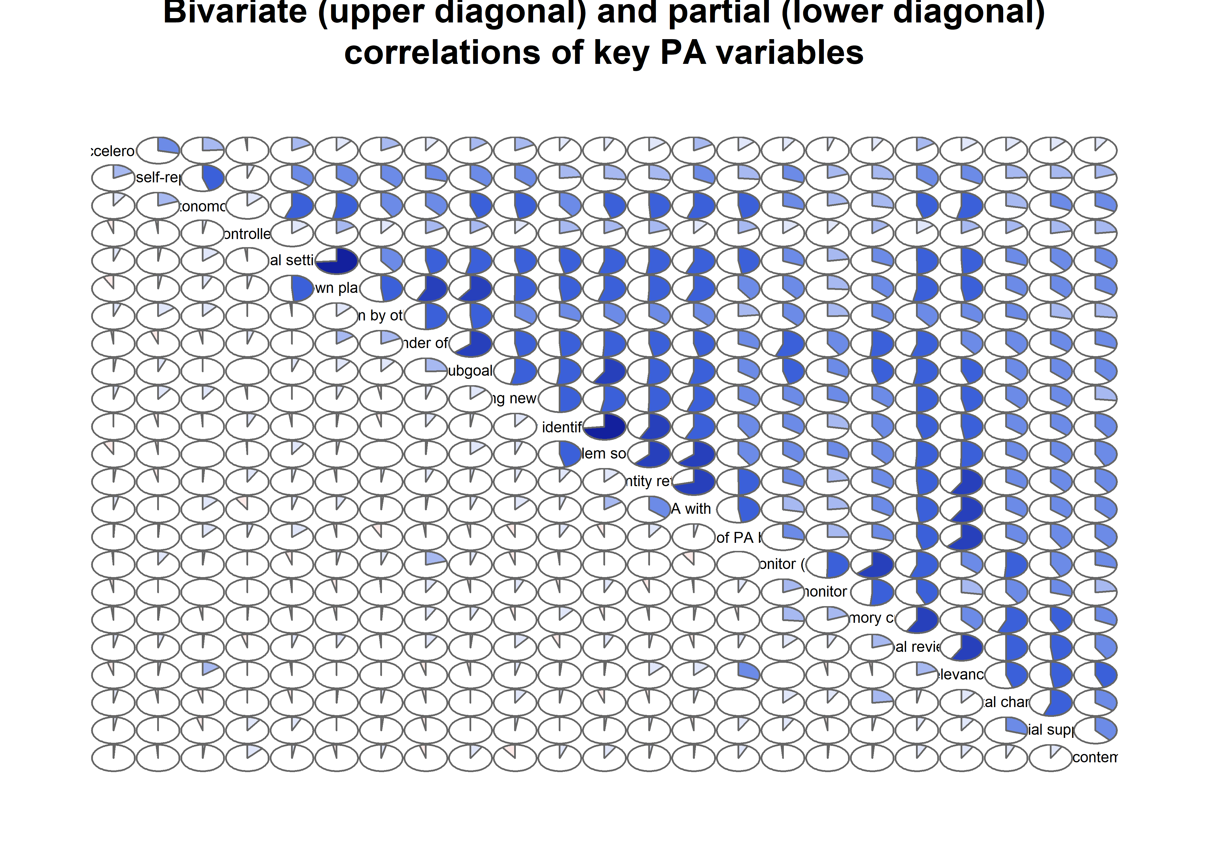
corMatrix_BCTs <- bivariate_BCTs %>% cor(use = "pairwise.complete.obs", method = "spearman")

as.data.frame(as.table(corMatrix_BCTs)) %>%
  dplyr::filter(Var1 == "PA accelerometer" | Var1 == "PA self report") %>%
  dplyr::mutate("Spearman correlation" = Freq %>% round(., 3) %>% format(., nsmall = 3)) %>%
  dplyr::select(-Freq) %>%
  dplyr::filter(`Spearman correlation` != 1) %>%
  dplyr::arrange(desc(`Spearman correlation`)) %>%
  DT::datatable(caption = "Bivariate correlations between BCTs, motivation and PA. Sorted by strength.")
Highest bivariate (Spearman) correlations with self-reported PA:
- I have tried out new ways for me to be physically active.
- I have personally made a specific plan (“what, where, how”) to implement my PA.
- I have a PA plan, which has been made by someone else, e.g. my sports club (e.g. a workout schedule).
- I have set PA goals for myself.
- I have broken down larger PA goals to smaller subgoals.
- I have compared my actualized PA with the PA goal I have set.
- I have attempted to find ways to exercise so, that it won’t obstruct but instead helps actualise my other life values.
- I have thought about which reasons to do PA are important to me personally.
- I have monitored my PA by marking the PA occasions on an exercise log on paper.
- I have a way by which I remind myself of my PA plan, e.g. I write it down in the calendar.
Prepare data and show correlation structure
bctdf_chunks <- df %>% dplyr::select(
  'agr-BCTs' = PA_agreementDependentBCT_T1,
  'frq-BCTs' = PA_frequencyDependentBCT_T1,
  'Accelerometer' = mvpaAccelerometer_T1,
  'Self-report' = padaysLastweek_T1,
  'intrinsic' = PA_intrinsic_T1,
  'identified' = PA_identified_T1,
  'introjected' = PA_introjected_T1,
  'extrinsic' = PA_extrinsic_T1) %>%
  rowwise() %>%
  mutate_all(as.numeric)

labs <- names(bctdf_chunks)

bctdf_chunks %>%
  corrgram::corrgram(
         cor.method = "pearson",
         # diag.panel=panel.minmax,
         # lower.panel=panel.shade,
         # lower.panel=panel.ellipse,
         # lower.panel=panel.cor,
         upper.panel=corrgram::panel.conf,
         lower.panel=corrgram::panel.pie,
         outer.labels=list(
           bottom=list(labels=labs,cex=.75, srt=60),
           left=list(labels=labs,cex=.75, srt=30))
         )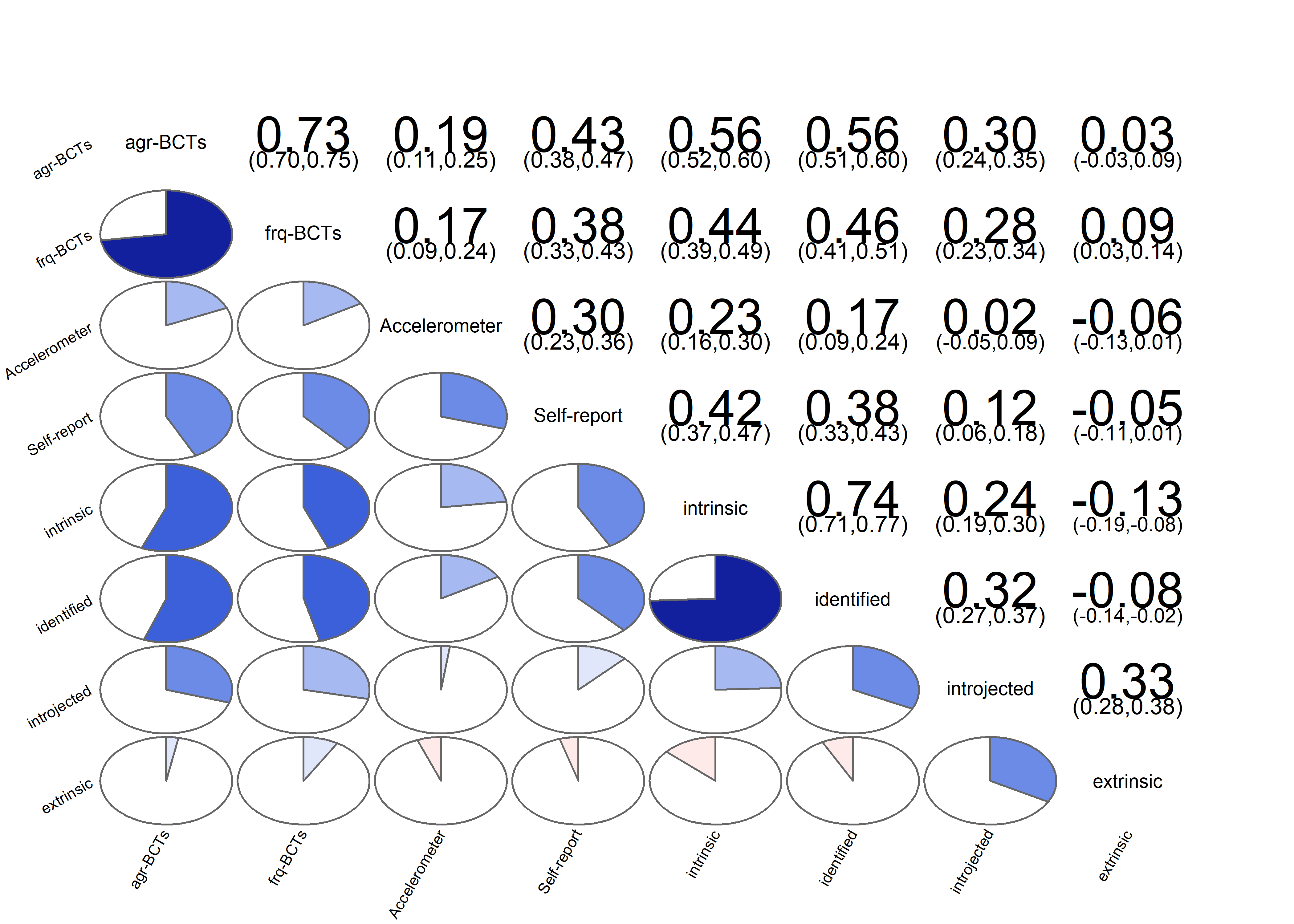
# Create a covariance matrix of the data
covMatrix <- bctdf_chunks %>% cov(use = "pairwise.complete.obs")

# Transform the matrix so, that lower diagonal of the matrix shows partial correlations,
# while the upper one shows bivariate correlations.
matrix_corLower_parcorUpper <- covMatrix %>% ggm::correlations()

# Show the matrix
matrix_corLower_parcorUpper %>%
papaja::apa_table(caption = "Correlation matrix of key variables of interest. Lower diagonal shows bivariate correlations, upper diagonal shows partial correlations")| agr-BCTs | frq-BCTs | Accelerometer | Self-report | intrinsic | identified | introjected | extrinsic | |
|---|---|---|---|---|---|---|---|---|
| agr-BCTs | 1.00 | 0.59 | 0.01 | 0.12 | 0.19 | 0.12 | 0.07 | 0.01 |
| frq-BCTs | 0.73 | 1.00 | 0.02 | 0.10 | -0.01 | 0.06 | 0.06 | 0.08 |
| Accelerometer | 0.18 | 0.16 | 1.00 | 0.20 | 0.10 | -0.03 | -0.03 | -0.02 |
| Self-report | 0.43 | 0.38 | 0.29 | 1.00 | 0.14 | 0.05 | -0.03 | -0.01 |
| intrinsic | 0.56 | 0.44 | 0.23 | 0.42 | 1.00 | 0.59 | 0.03 | -0.13 |
| identified | 0.55 | 0.46 | 0.16 | 0.38 | 0.74 | 1.00 | 0.18 | -0.07 |
| introjected | 0.30 | 0.28 | 0.02 | 0.12 | 0.24 | 0.32 | 1.00 | 0.36 |
| extrinsic | 0.03 | 0.09 | -0.06 | -0.05 | -0.13 | -0.08 | 0.33 | 1.00 |
# Plot the matrix as a correlogram
matrix_corLower_parcorUpper %>% corrgram::corrgram(
  type = "cor",
  lower.panel = corrgram::panel.pie,
  upper.panel = corrgram::panel.pie,
  main = "Bivariate (upper diagonal) and partial (lower diagonal)\ncorrelations of key PA variables")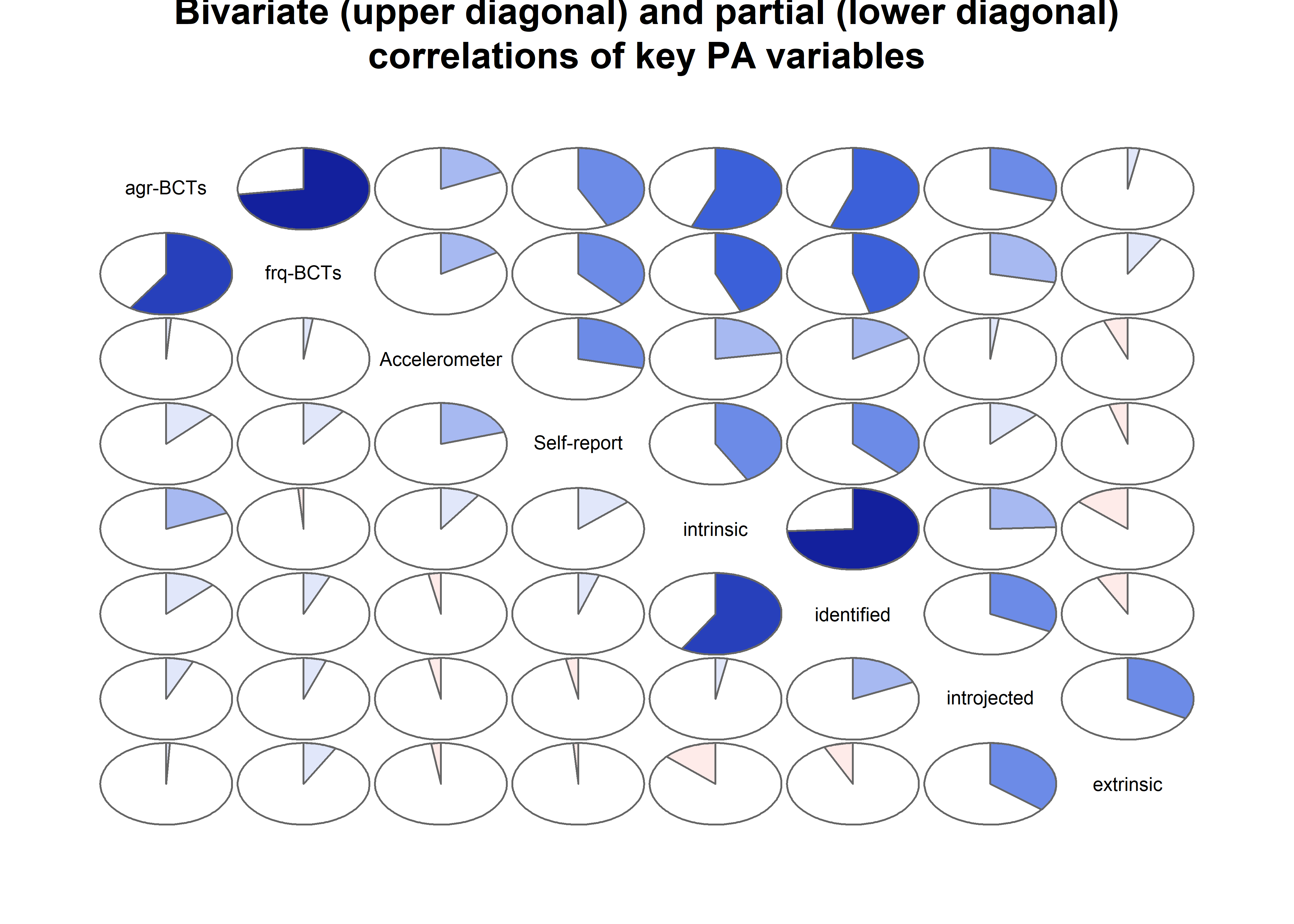
Estimate and plot networks
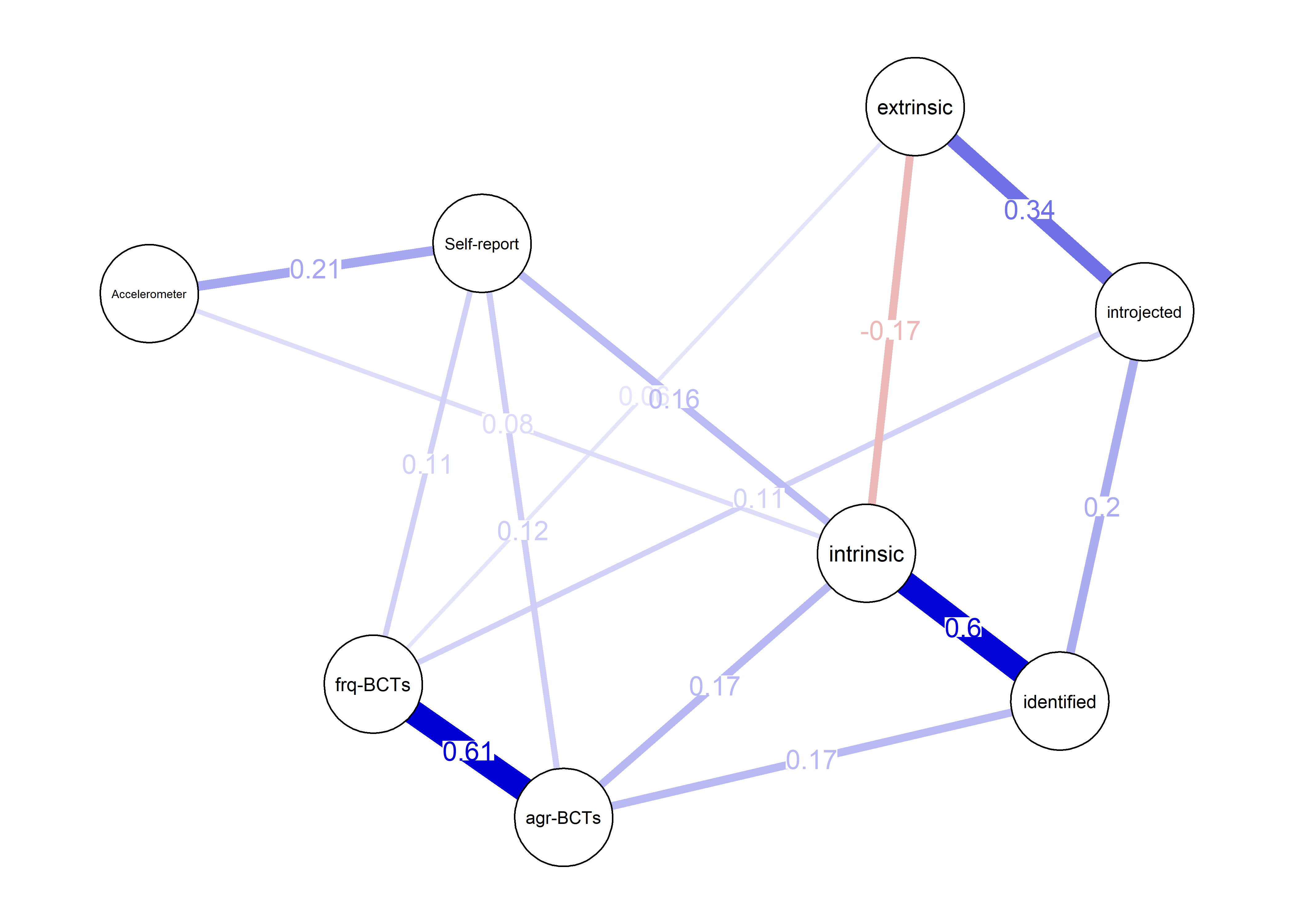
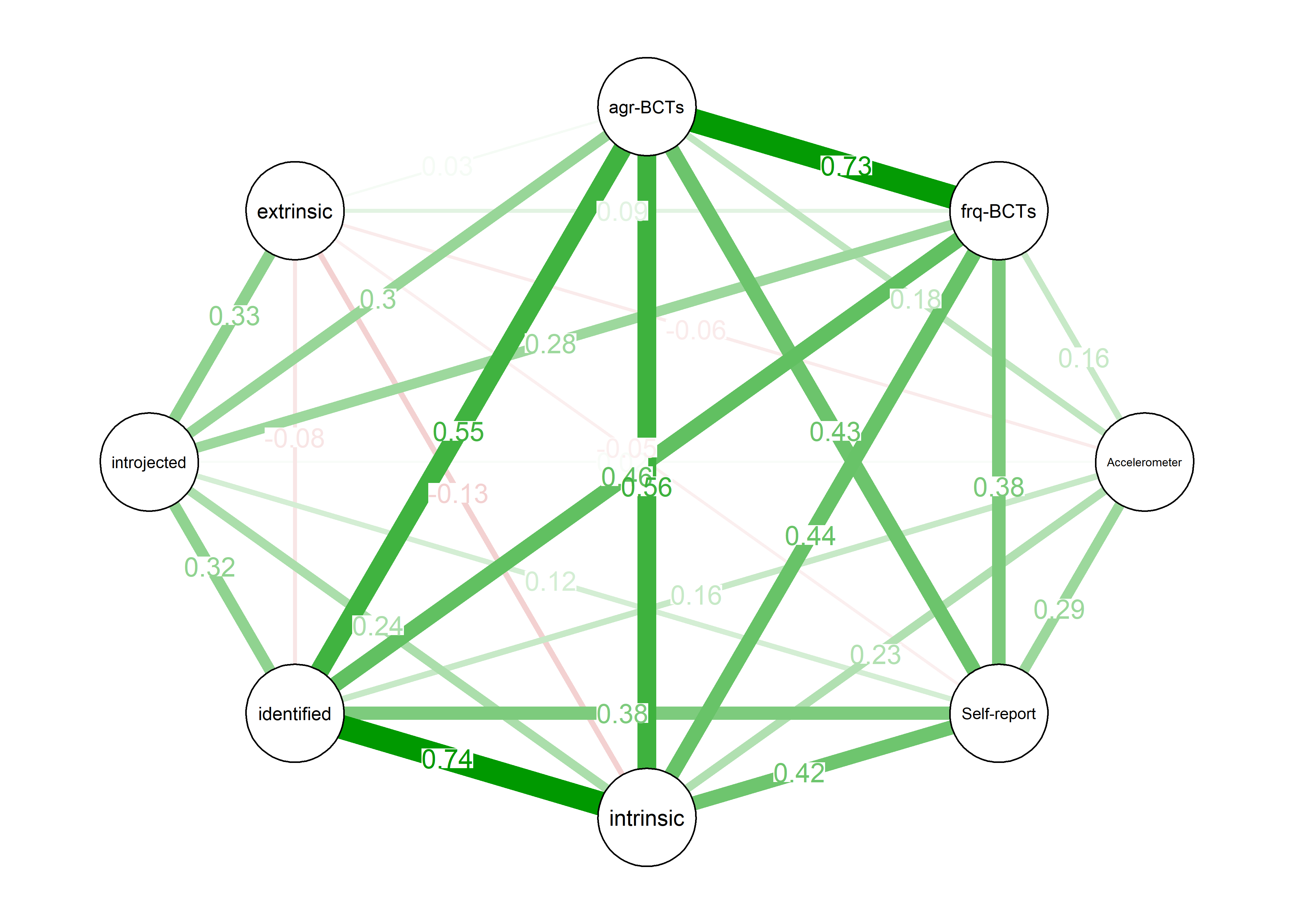
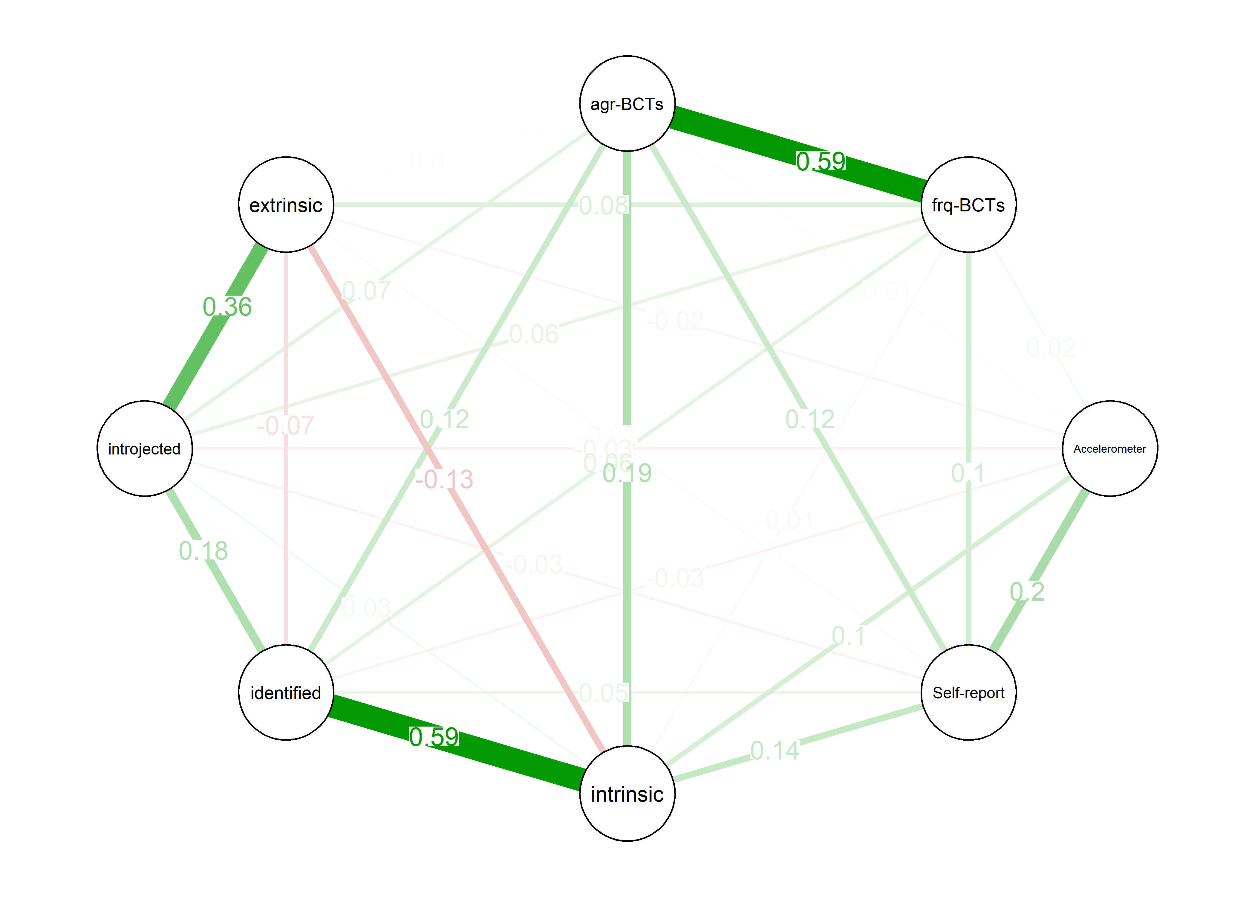
# Average the layout according to three previous plots, and plot each according to the layout
avlayout <- qgraph::averageLayout(bootnetgraph, corgraph, pcorgraph)

corgraph <- qgraph::qgraph(qgraph::cor_auto(bctdf_chunks), graph = "cor",
       labels = names(bctdf_chunks),
       edge.labels = TRUE,
       layout = avlayout,
       title = "bivariate correlation network",
       theme = "colorblind",
       maximum = max(c(bootnetgraph$graph$Graph$maximum,
                     pcorgraph$graph$Graph$maximum,
                     corgraph$graph$Graph$maximum)))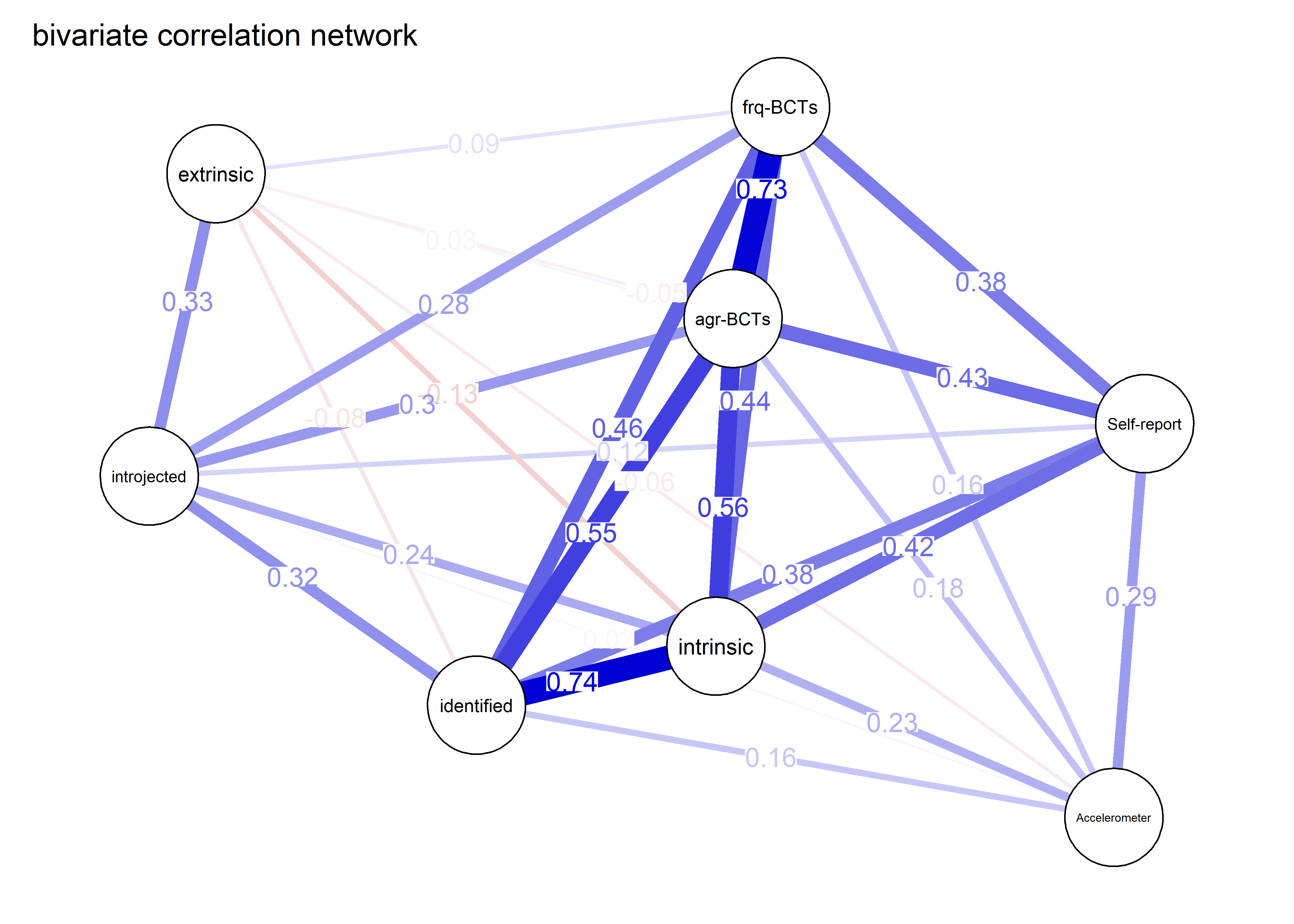
# To help with visual comparison, that last argument takes the maximum edge of the three
# graphs and places that as the benchmark for the thickest line in all plots.

pcorgraph <- qgraph::qgraph(qgraph::cor_auto(bctdf_chunks), graph = "pcor",
       labels = names(bctdf_chunks),
       edge.labels = TRUE,
       layout = avlayout,
       title = "partial correlation network",
       theme = "colorblind",
       maximum = max(c(bootnetgraph$graph$Graph$maximum,
                     pcorgraph$graph$Graph$maximum,
                     corgraph$graph$Graph$maximum)))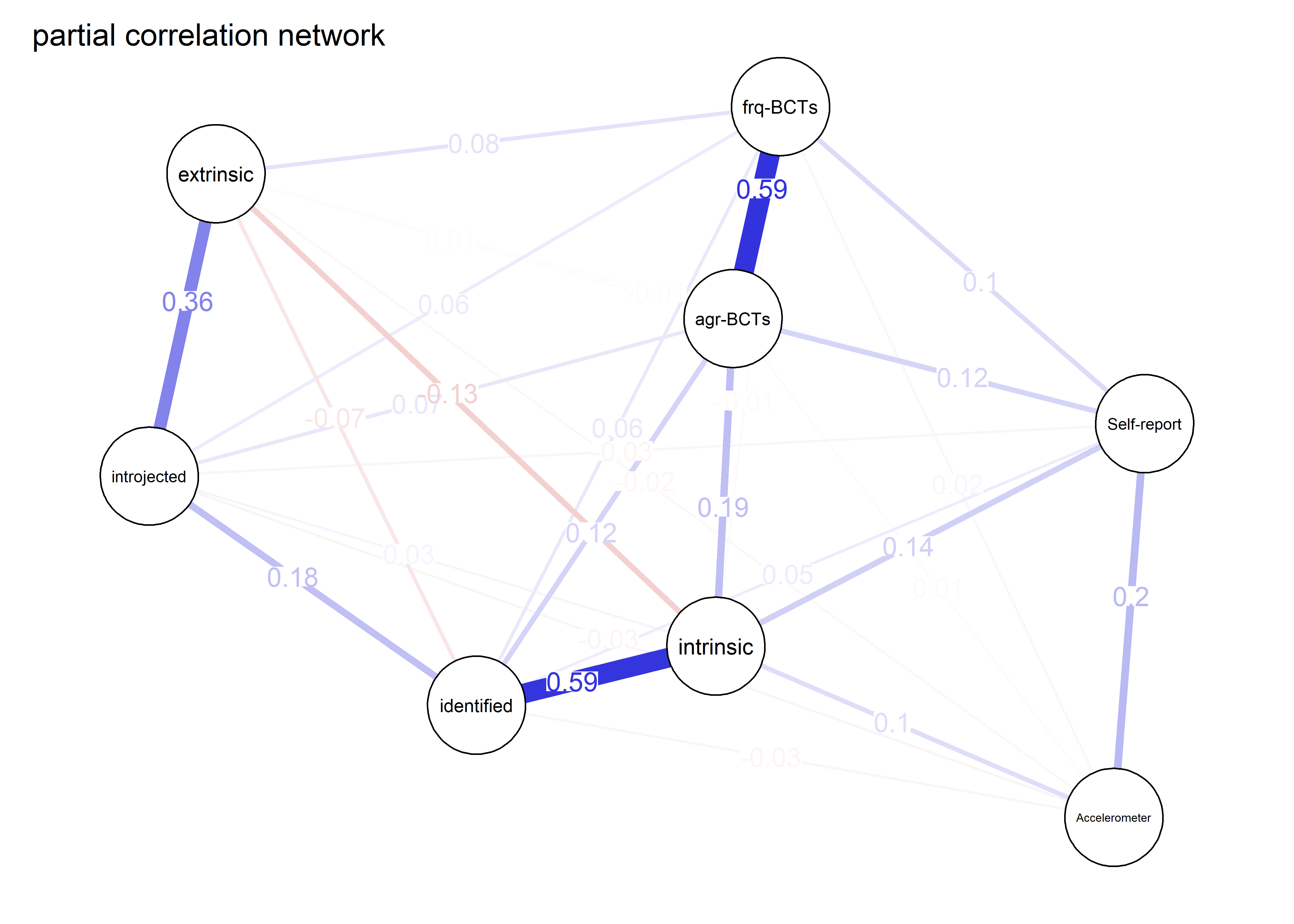
bootnetgraph <- plot(nwBCT_chunks,
                     edge.labels = TRUE,
                     layout = avlayout,
                     title = "ggmModSelect",
       maximum = max(c(bootnetgraph$graph$Graph$maximum,
                     pcorgraph$graph$Graph$maximum,
                     corgraph$graph$Graph$maximum)))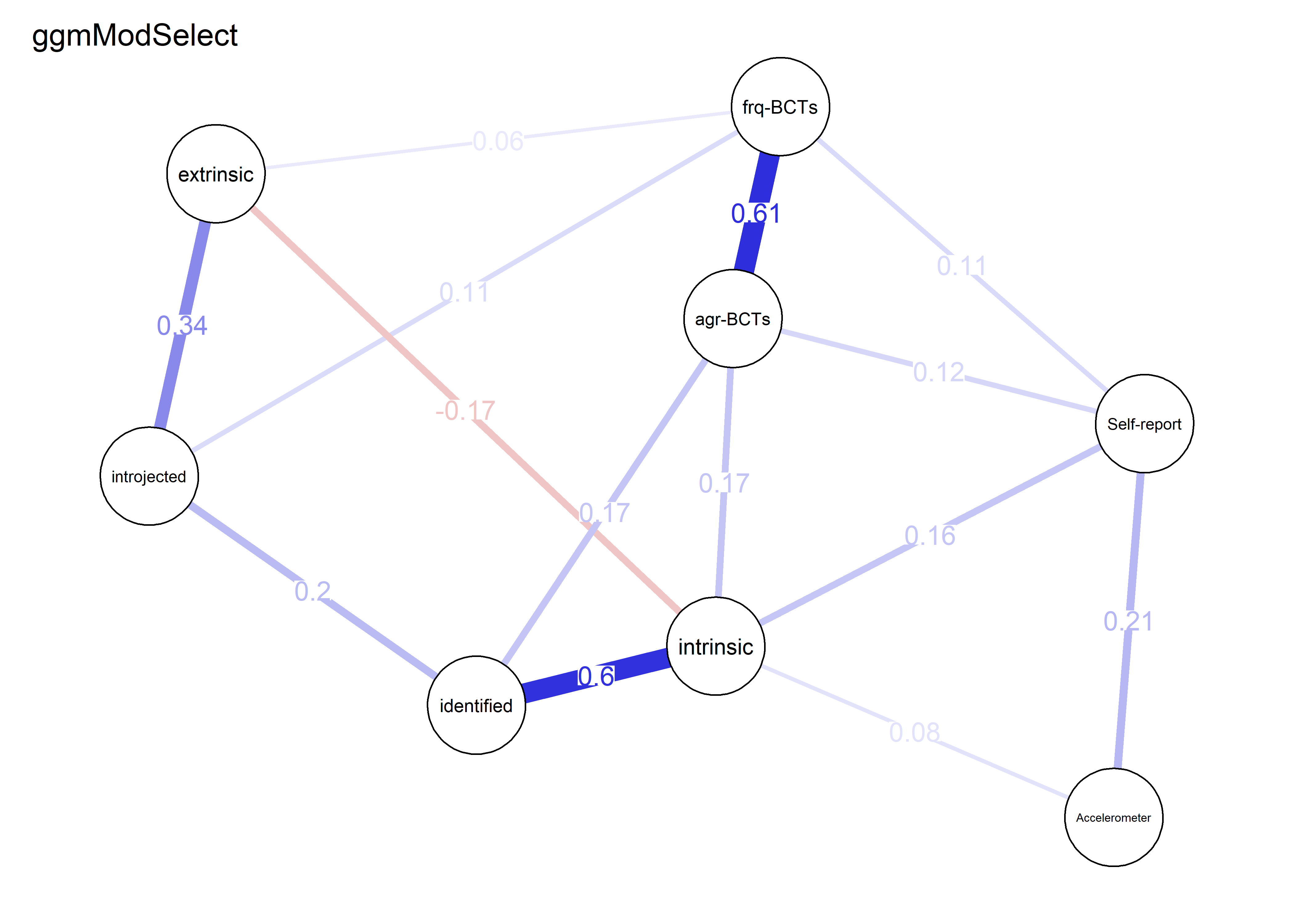
Stability
# bootnet_stability_output <- bootnet::bootnet(nwBCT_chunks, nBoots=1000)
# save(bootnet_stability_output, file = "./Rdata_files/bootnet_stability_output.Rdata")
load("./Rdata_files/bootnet_stability_output.Rdata")

plot(bootnet_stability_output, labels = TRUE, order = "sample") 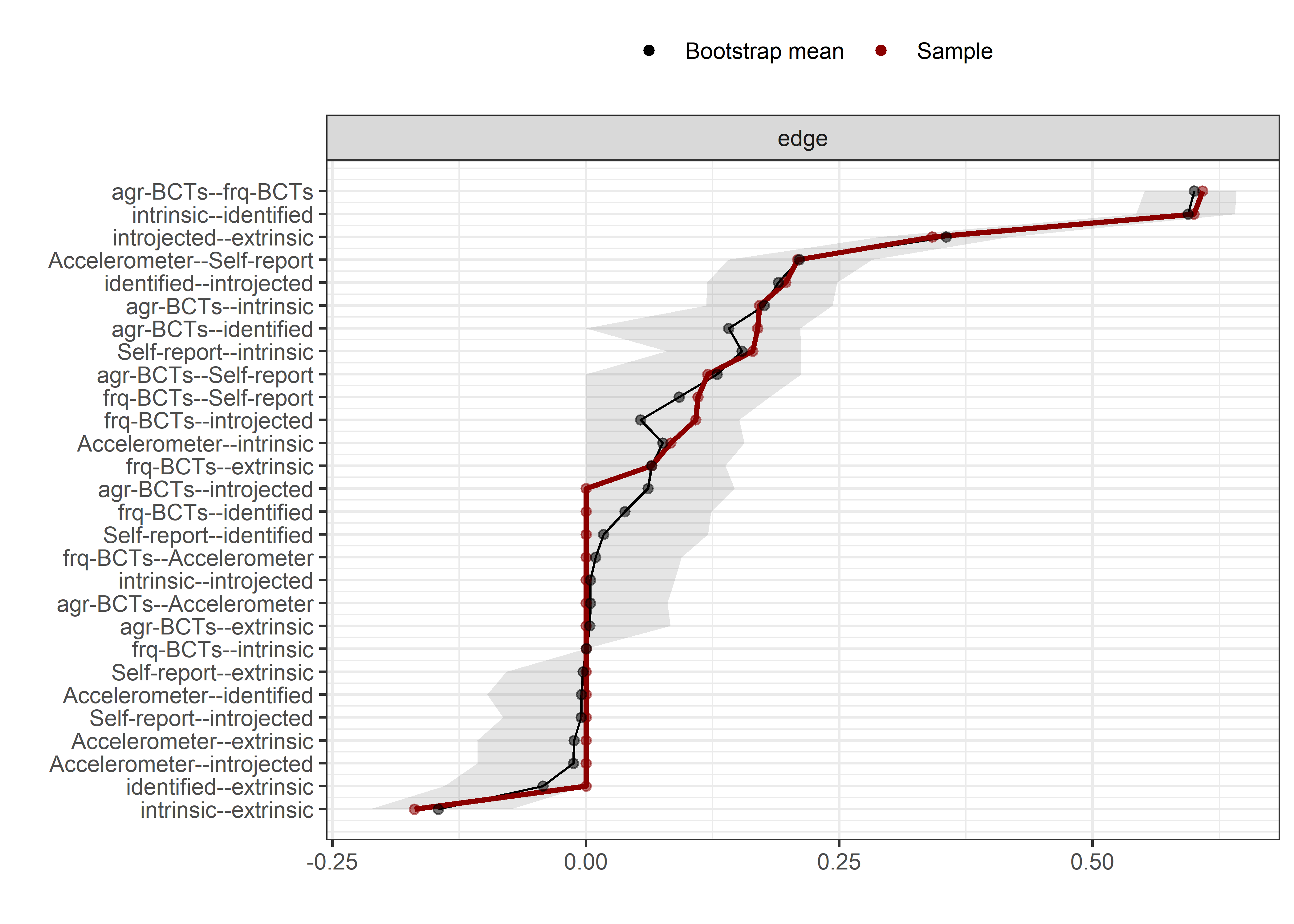
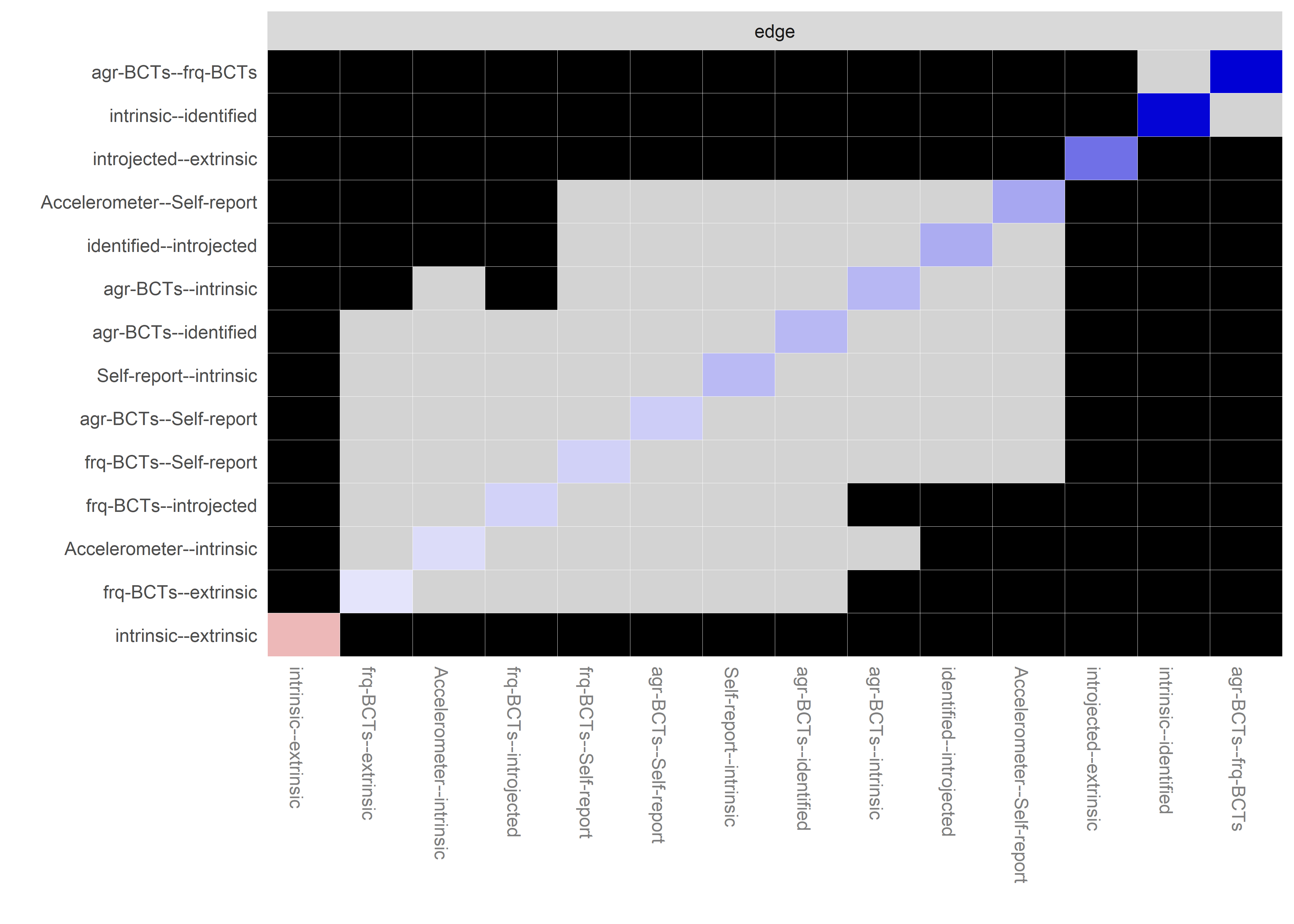
# bootnet_centrality_stability_output <- bootnet::bootnet(nwBCT_chunks, nBoots=1000,nCores=8, type="case")
# save(bootnet_centrality_stability_output, file = "./Rdata_files/bootnet_centrality_stability_output.Rdata")
load("./Rdata_files/bootnet_centrality_stability_output.Rdata")

plot(bootnet_centrality_stability_output)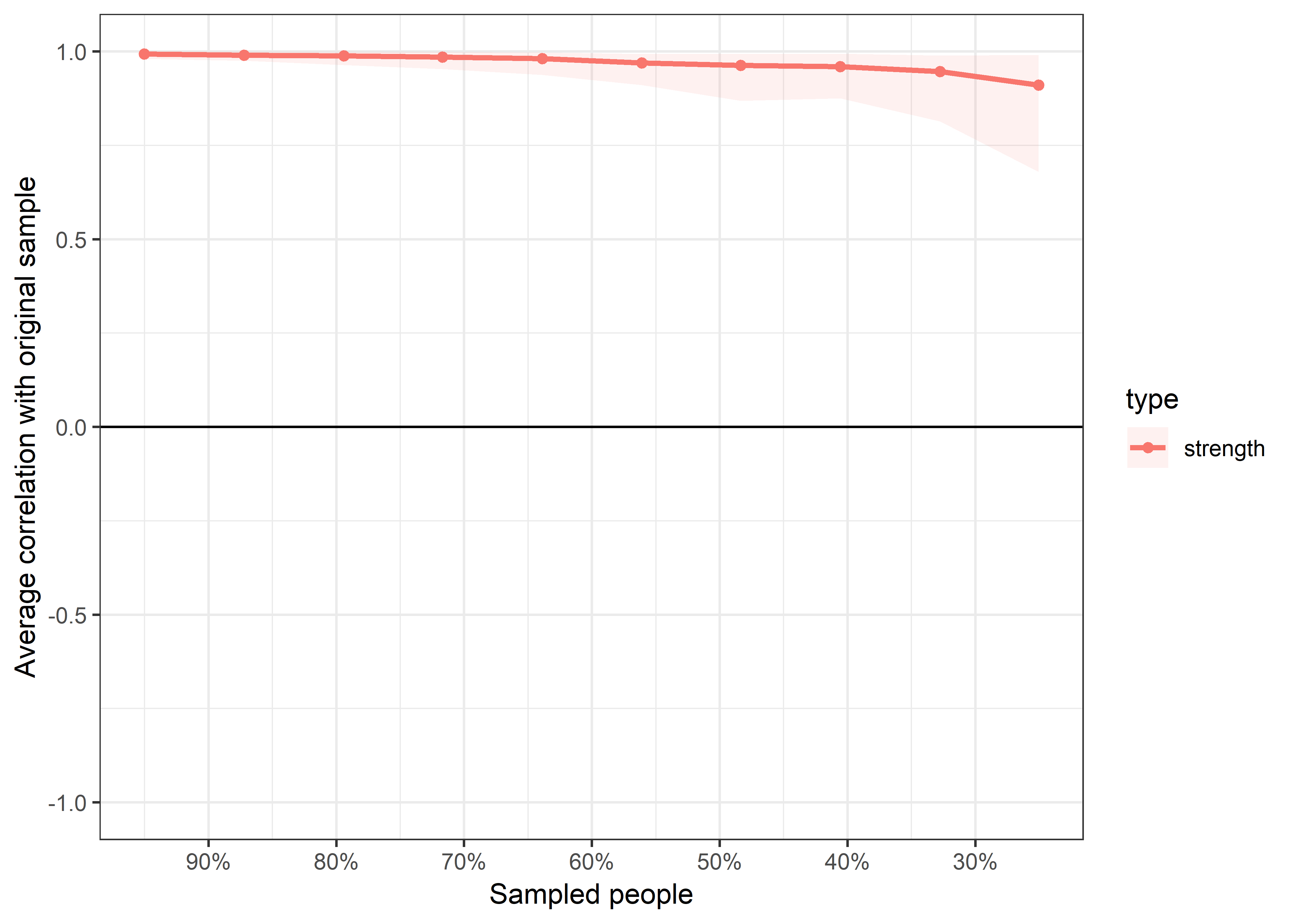
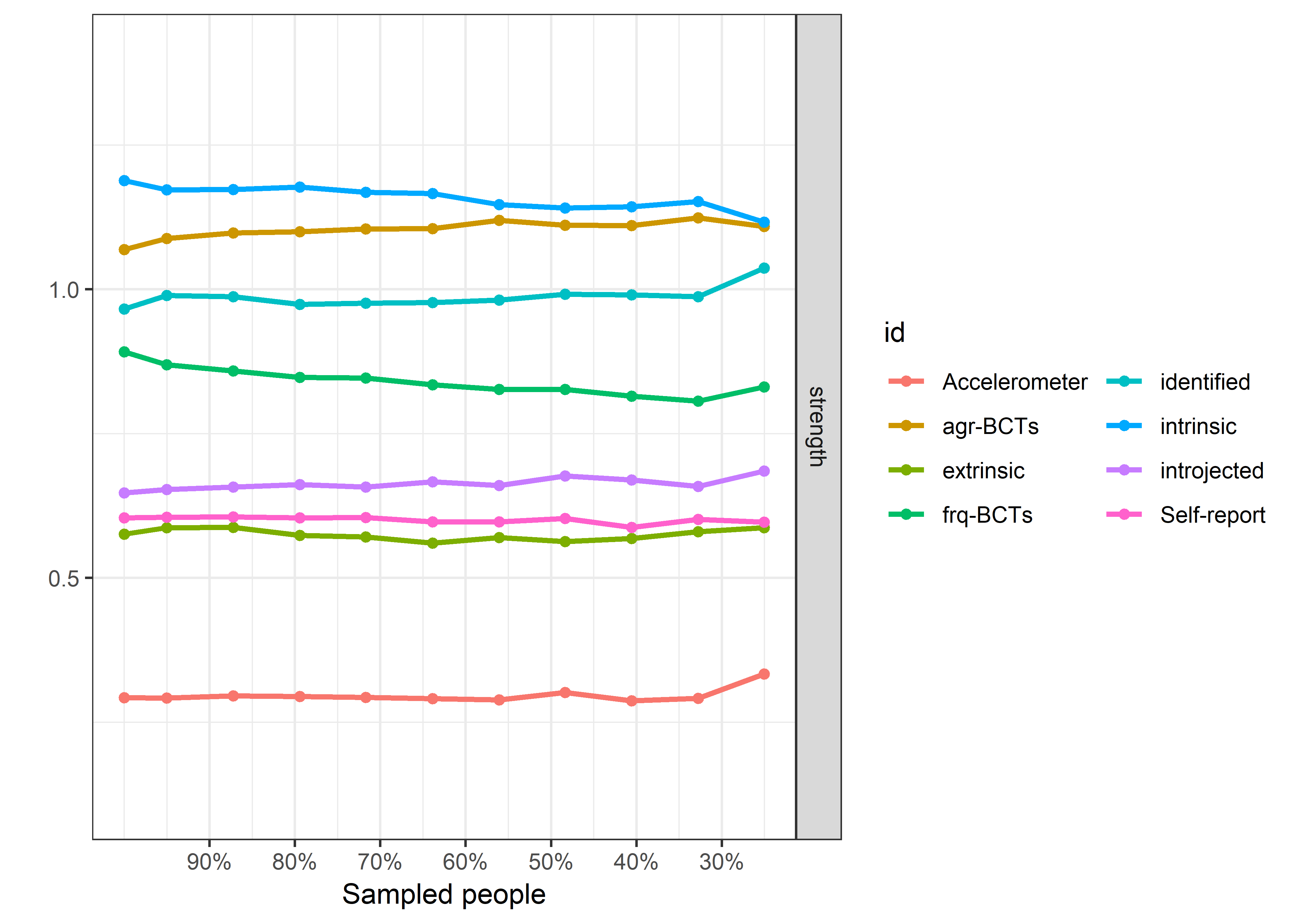
Individual agreement-related BCTs and PA
Network without combining nodes
bctdf_pa_mgm <- df %>% dplyr::select(
#  id,
#  intervention,
#  group,
#  school,
  'PA selfrep' = padaysLastweek_T1,
  'PA accelerometer' = mvpaAccelerometer_T1,
  'goal setting' = PA_agreementDependentBCT_01_T1,
  'own plan' = PA_agreementDependentBCT_02_T1,
  'plan by other' = PA_agreementDependentBCT_03_T1,
  'reminder of plan' = PA_agreementDependentBCT_04_T1,
  'subgoals' = PA_agreementDependentBCT_05_T1,
  'trying new PA' = PA_agreementDependentBCT_06_T1,
  'barrier identification' = PA_agreementDependentBCT_07_T1,
  'problem solving' = PA_agreementDependentBCT_08_T1,
  'PA identity reflection' = PA_agreementDependentBCT_09_T1,
  'aligning PA with life values' = PA_agreementDependentBCT_10_T1) %>%
 rowwise() %>%
 mutate(
  'goal setting' = ifelse(`goal setting` == 1, 0, 1),
  # 'has plan' = ifelse(`own plan` == 1 & `plan by other` == 1, 0, 1),
  'own plan' = ifelse(`own plan` == 1, 0, 1),
  'reminder of plan' = ifelse(`reminder of plan` == 1, 0, 1),
  'subgoals' = ifelse(`subgoals` == 1, 0, 1),
  'trying new PA' = ifelse(`trying new PA` == 1, 0, 1),
  'plan by other' = ifelse(`plan by other` == 1, 0, 1),
 'barrier identification' = ifelse(`barrier identification` == 1, 0, 1),
 'problem solving' = ifelse(`problem solving` == 1, 0, 1),
  # 'barriers identified or planned for' = ifelse(`problem solving` == 1 & `barrier identification` == 1, 0, 1),
 'PA identity reflection' = ifelse(`PA identity reflection` == 1, 0, 1),
 'aligning PA with life values' = ifelse(`aligning PA with life values` == 1, 0, 1)) %>%
  # 'identity, life values' = ifelse(`PA identity reflection` == 1 & `aligning PA with life values` == 1, 0, 1),
  # dplyr::select(-`self-monitor (paper)`, -`self-monitor (app)`, -`plan by other`, -`own plan`, -identified, -intrinsic,
  #        -`failure contemplated`, # only concerns those who haven't reached goals
  #        -`barrier identification`, -`problem solving`, # closely related
  #        -`PA identity reflection`, -`aligning PA with life values`) %>% # closely related
#  dplyr::select(-controlled) %>% # Not really gaussian at all
  # data.frame %>%
  mutate_all(as.numeric)

# bctdf_mgm$autonomous[is.nan(bctdf_mgm$autonomous)] <- NA

# Create a covariance matrix of the data
covMatrix <- bctdf_pa_mgm %>% cov(use = "pairwise.complete.obs")

# Transform the matrix so, that lower diagonal of the matrix shows partial correlations,
# while the upper one shows bivariate correlations.
matrix_corLower_parcorUpper <- covMatrix %>% ggm::correlations()

# Show the matrix
matrix_corLower_parcorUpper %>% papaja::apa_table(caption = "Correlation matrix of key variables of interest. Lower diagonal shows bivariate correlations, upper diagonal shows partial correlations")| PA selfrep | PA accelerometer | goal setting | own plan | plan by other | reminder of plan | subgoals | trying new PA | barrier identification | problem solving | PA identity reflection | aligning PA with life values | |
|---|---|---|---|---|---|---|---|---|---|---|---|---|
| PA selfrep | 1.00 | 0.23 | 0.01 | 0.06 | 0.15 | 0.00 | 0.03 | 0.14 | -0.03 | -0.03 | 0.02 | 0.03 |
| PA accelerometer | 0.29 | 1.00 | 0.05 | 0.00 | 0.05 | -0.05 | 0.02 | 0.04 | -0.02 | -0.08 | 0.05 | 0.02 |
| goal setting | 0.26 | 0.14 | 1.00 | 0.51 | -0.02 | 0.02 | 0.00 | 0.07 | 0.07 | 0.10 | 0.06 | 0.03 |
| own plan | 0.30 | 0.13 | 0.71 | 1.00 | 0.13 | 0.09 | 0.15 | 0.05 | -0.03 | 0.06 | -0.04 | 0.09 |
| plan by other | 0.32 | 0.14 | 0.38 | 0.47 | 1.00 | 0.28 | 0.15 | 0.00 | 0.05 | -0.01 | -0.01 | 0.03 |
| reminder of plan | 0.25 | 0.07 | 0.45 | 0.52 | 0.56 | 1.00 | 0.32 | 0.10 | 0.11 | 0.03 | 0.02 | -0.04 |
| subgoals | 0.29 | 0.12 | 0.50 | 0.58 | 0.52 | 0.64 | 1.00 | 0.13 | 0.01 | 0.14 | 0.04 | 0.05 |
| trying new PA | 0.32 | 0.15 | 0.47 | 0.48 | 0.38 | 0.48 | 0.52 | 1.00 | 0.10 | 0.03 | 0.07 | 0.14 |
| barrier identification | 0.20 | 0.06 | 0.50 | 0.48 | 0.40 | 0.50 | 0.52 | 0.51 | 1.00 | 0.46 | 0.14 | 0.07 |
| problem solving | 0.21 | 0.05 | 0.54 | 0.53 | 0.39 | 0.50 | 0.57 | 0.51 | 0.74 | 1.00 | 0.15 | 0.15 |
| PA identity reflection | 0.24 | 0.13 | 0.47 | 0.45 | 0.35 | 0.42 | 0.49 | 0.49 | 0.59 | 0.62 | 1.00 | 0.42 |
| aligning PA with life values | 0.26 | 0.12 | 0.49 | 0.50 | 0.37 | 0.42 | 0.51 | 0.53 | 0.58 | 0.62 | 0.69 | 1.00 |
# Plot the matrix as a correlogram
matrix_corLower_parcorUpper %>% corrgram::corrgram(
  type = "cor",
  lower.panel = corrgram::panel.pie,
  upper.panel = corrgram::panel.pie,
  main = "Bivariate (upper diagonal) and partial (lower diagonal)\ncorrelations of agreement-BCTs and PA")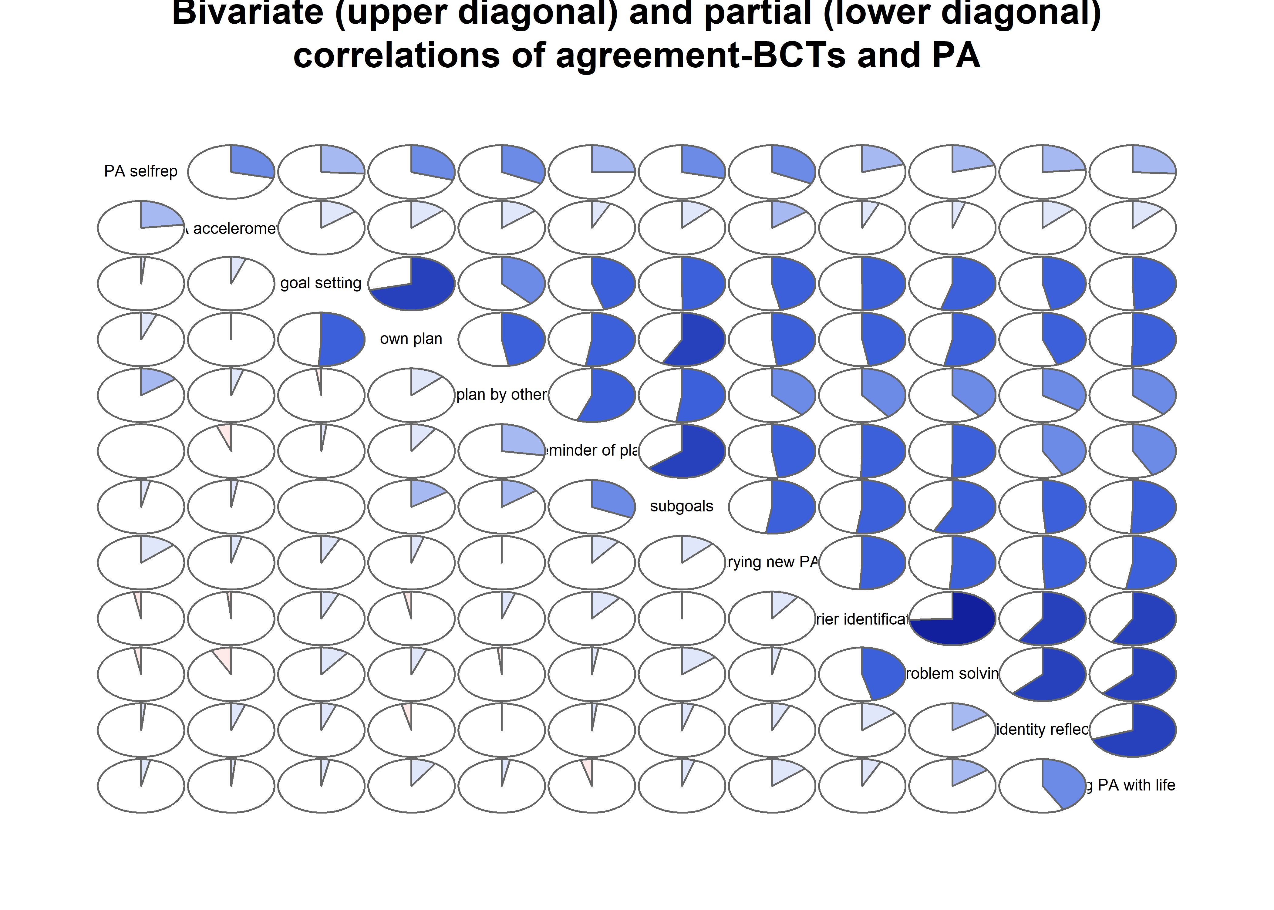
mgm estimation
# devtools::install_github("jmbh/mgm")
# Restart R for the latest package
# .r.restartR()

# mgm wants full data, see package missForest for imputation
bctdf_pa_mgm_fullobs <- bctdf_pa_mgm %>% na.omit()

mgm_pa_variable_types <- c("c", "g", rep("c", 10))
mgm_pa_variable_levels <- c("8", "1", rep("2", 10))
# data.frame(mgm_pa_variable_types, mgm_pa_variable_levels, names(bctdf_pa_mgm_fullobs))

mgm_obj <- mgm::mgm(data = bctdf_pa_mgm_fullobs,
  type = mgm_pa_variable_types,
  level = mgm_pa_variable_levels,
  lambdaSel = "CV",
  lambdaFolds = 10,
  pbar = FALSE,
  binarySign = TRUE)
## Note that the sign of parameter estimates is stored separately; see ?mgm

pred_obj <- predict(object = mgm_obj,
                         data = bctdf_pa_mgm_fullobs)

pred_obj$errors
# Take R2 from gaussian, CC from categorical variables
pie_errors <- c(pred_obj$errors[1, 4],
                pred_obj$errors[2, 3],
                pred_obj$errors[3:nrow(pred_obj$errors), 4])

# PLOT NETWORK

node_colors <- c(viridis::viridis(4, begin = 0.3, end = 0.8)[1],
                 viridis::viridis(4, begin = 0.3, end = 0.8)[2],
                 rep(viridis::viridis(4, begin = 0.3, end = 0.8)[3], 10))

BCT_mgm <- qgraph::qgraph(mgm_obj$pairwise$wadj,
            layout = "spring",
            repulsion = 0.90, # To nudge the network from originally bad visual state
            title = "agreement-measured BCTs and PA (accelerometer & self-reported)",
            edge.color = ifelse(mgm_obj$pairwise$edgecolor == "darkgreen", "blue", mgm_obj$pairwise$edgecolor),
            pie = pie_errors,
            pieColor = viridis::viridis(4, begin = 0.3, end = 0.8)[4],
            color = node_colors,
            labels = names(bctdf_pa_mgm_fullobs),
            label.cex = 0.75,
            label.scale = FALSE,
            label.color = c(rep("black", 12)))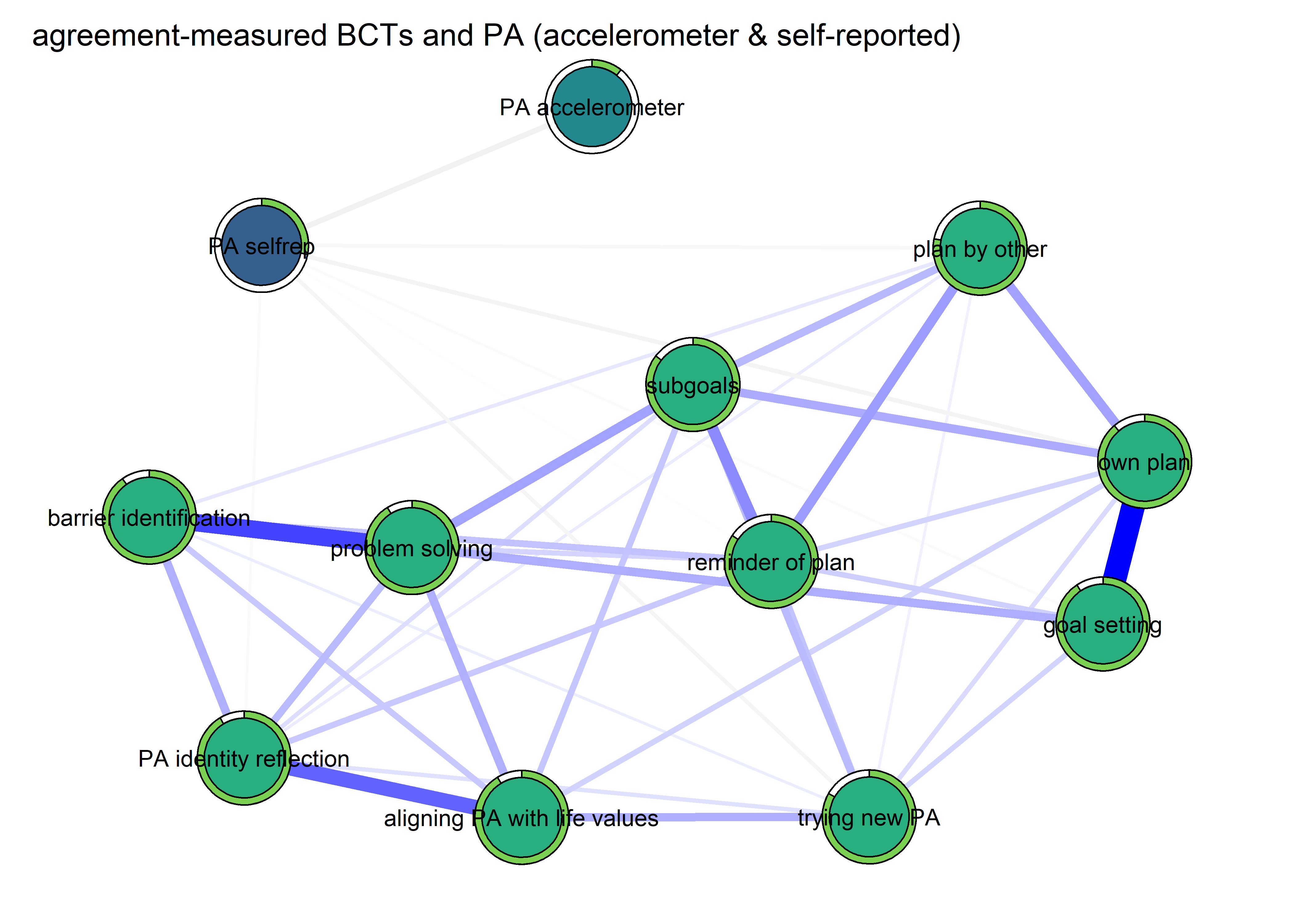
ggm estimation
# Estimate a network

individualAgreementBCTs <- bootnet::estimateNetwork(bctdf_pa_mgm, default="ggmModSelect")

bootnetgraph <- plot(individualAgreementBCTs, edge.labels = TRUE,
       title = "ggmModSelect")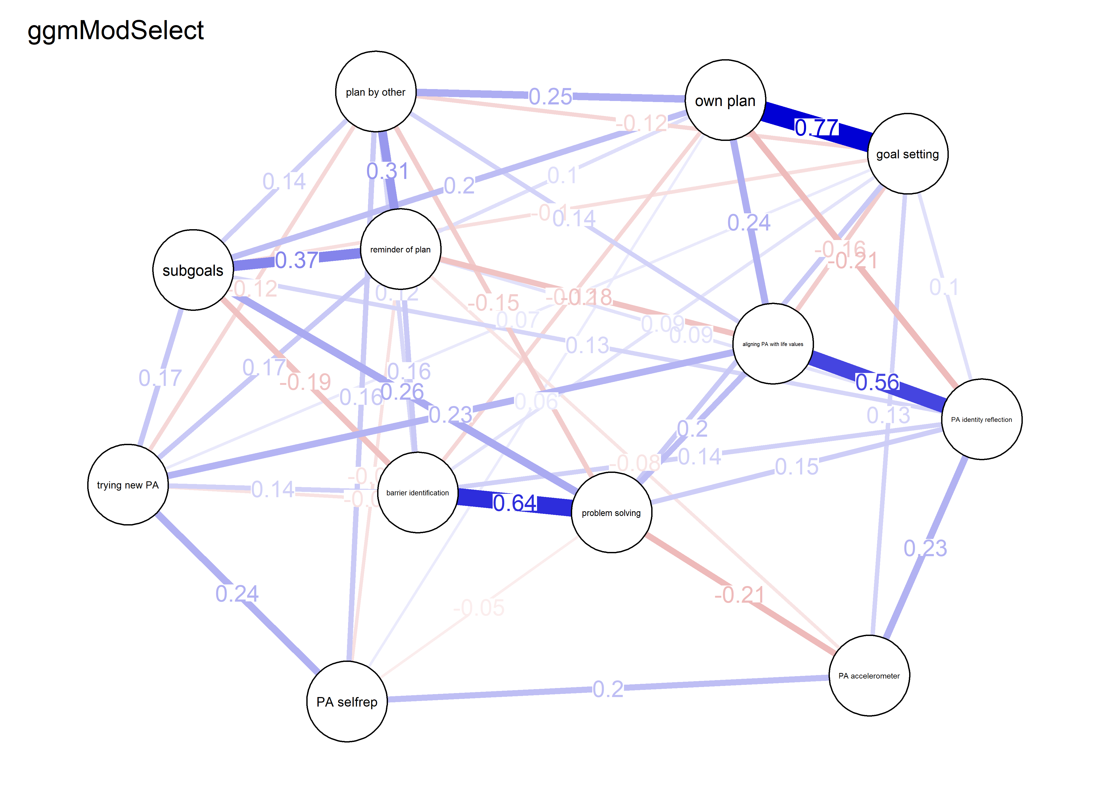
corgraph <- qgraph::qgraph(qgraph::cor_auto(bctdf_pa_mgm), graph = "cor",
       labels = names(bctdf_pa_mgm),
       edge.labels = TRUE,
       title = "bivariate correlation network")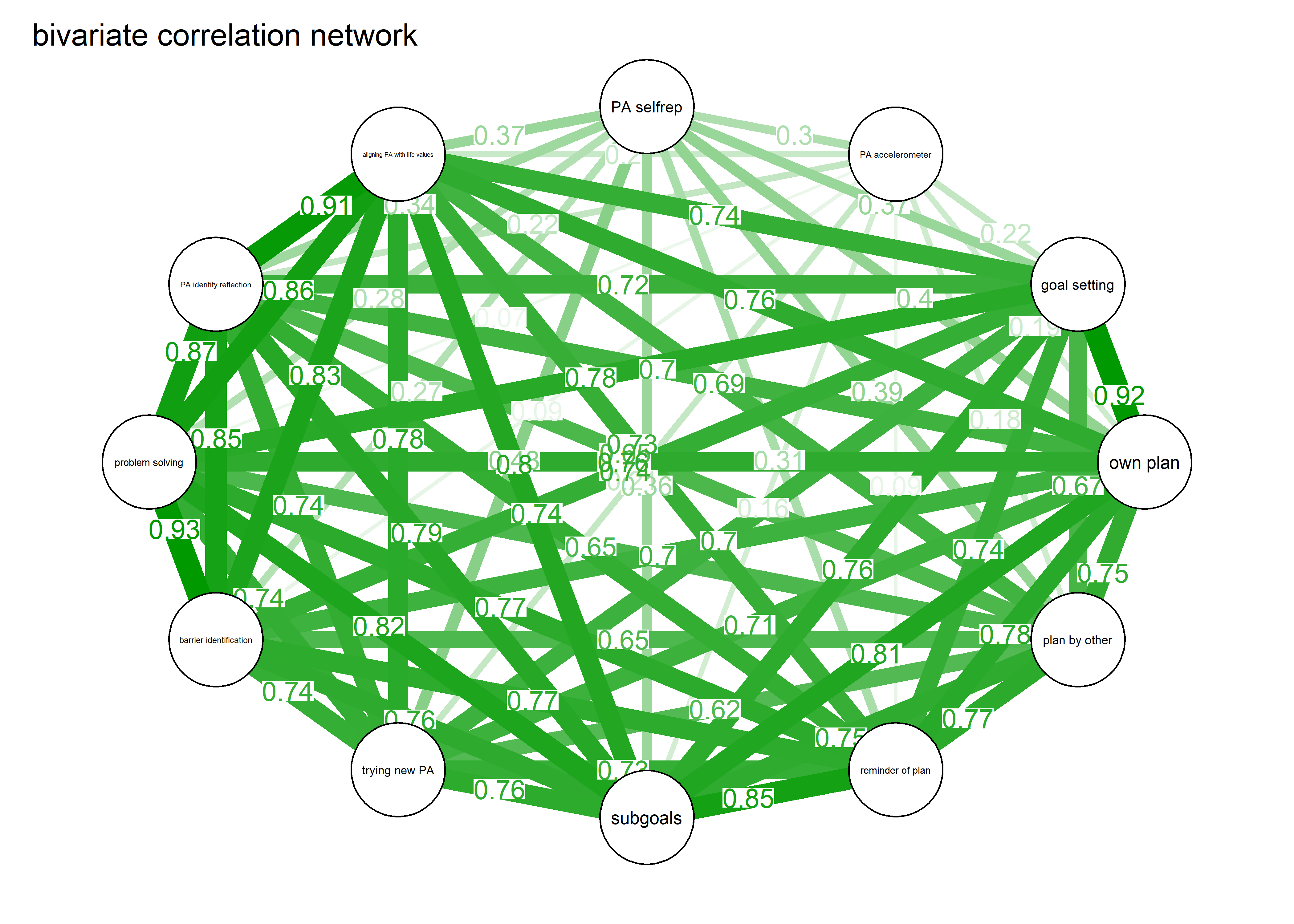
pcorgraph <- qgraph::qgraph(qgraph::cor_auto(bctdf_pa_mgm), graph = "pcor",
       labels = names(bctdf_pa_mgm),
       edge.labels = TRUE,
       title = "partial correlation network")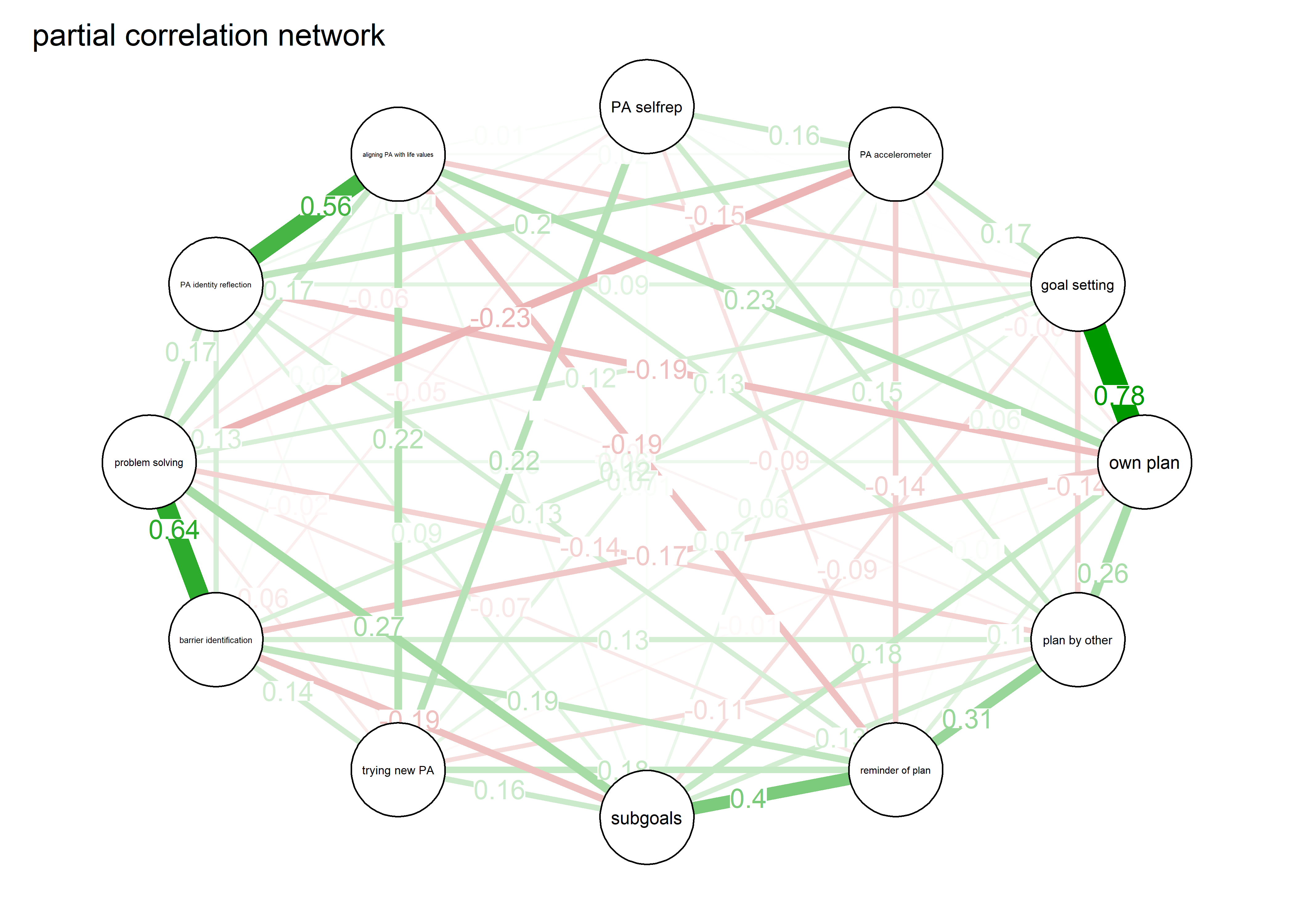
# Average the layout and plot all according to that
avlayout <- qgraph::averageLayout(bootnetgraph, corgraph, pcorgraph)

corgraph <- qgraph::qgraph(qgraph::cor_auto(bctdf_pa_mgm), graph = "cor",
       labels = names(bctdf_pa_mgm),
       edge.labels = TRUE,
       layout = avlayout,
       title = "bivariate correlation network",
       theme = "colorblind",
       maximum = max(c(bootnetgraph$graph$Graph$maximum,
                     pcorgraph$graph$Graph$maximum,
                     corgraph$graph$Graph$maximum)),
       label.scale = FALSE)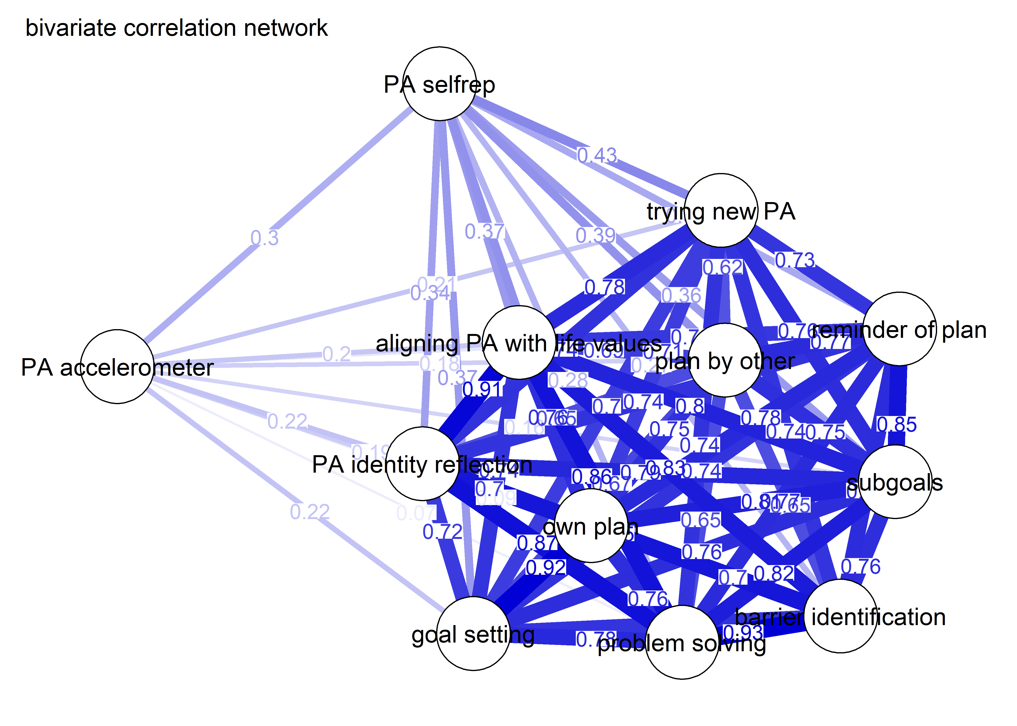
# To help with visual comparison, that last argument takes the maximum edge of the three
# graphs and places that as the benchmark for the thickest line in all plots.

pcorgraph <- qgraph::qgraph(qgraph::cor_auto(bctdf_pa_mgm), graph = "pcor",
       labels = names(bctdf_pa_mgm),
       edge.labels = TRUE,
       layout = avlayout,
       title = "partial correlation network",
       theme = "colorblind",
       maximum = max(c(bootnetgraph$graph$Graph$maximum,
                     pcorgraph$graph$Graph$maximum,
                     corgraph$graph$Graph$maximum)),
       label.scale = FALSE)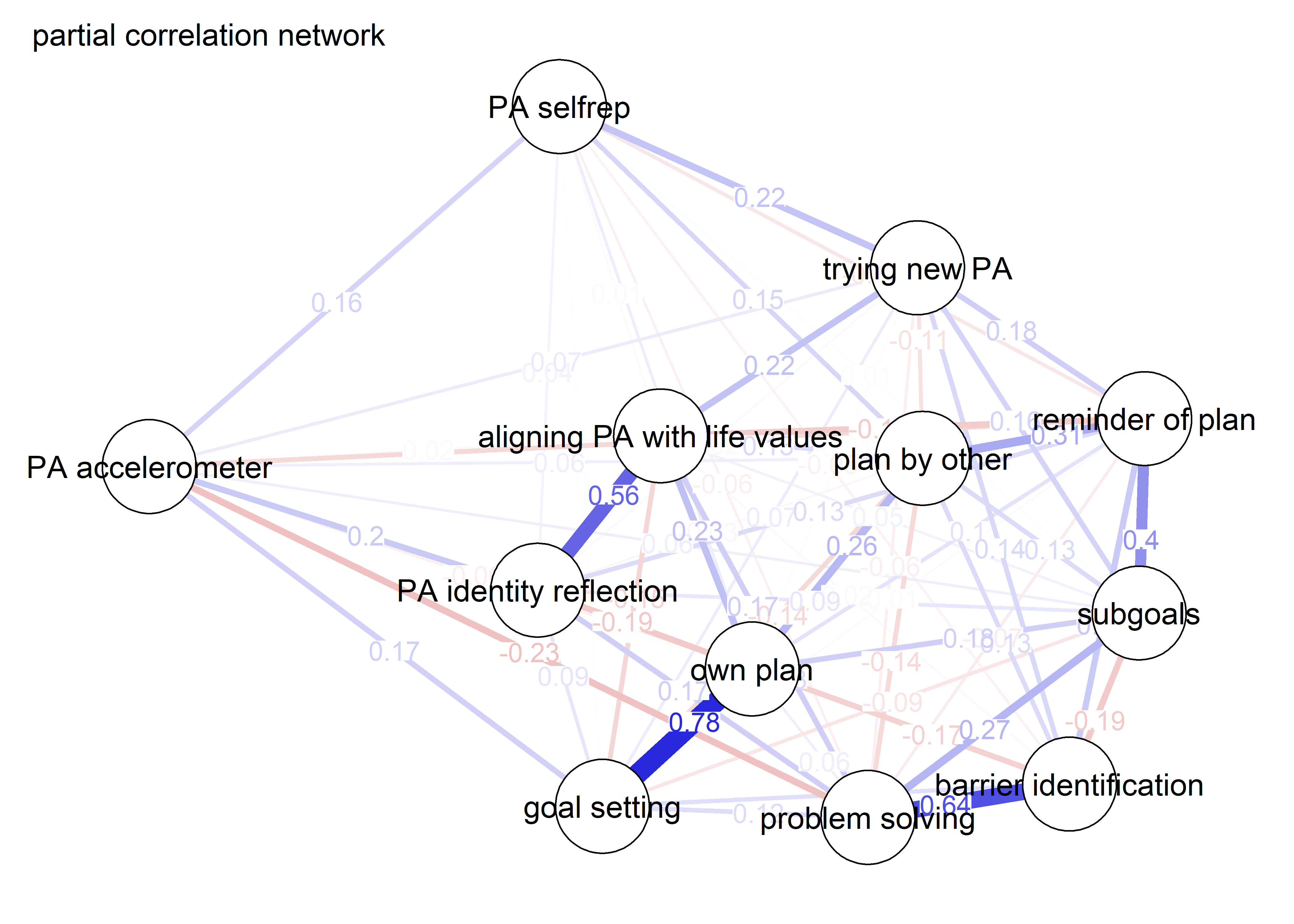
bootnetgraph <- plot(individualAgreementBCTs,
                     edge.labels = TRUE,
                     layout = avlayout,
                     title = "ggmModSelect",
       maximum = max(c(bootnetgraph$graph$Graph$maximum,
                     pcorgraph$graph$Graph$maximum,
                     corgraph$graph$Graph$maximum)),
       label.scale = FALSE)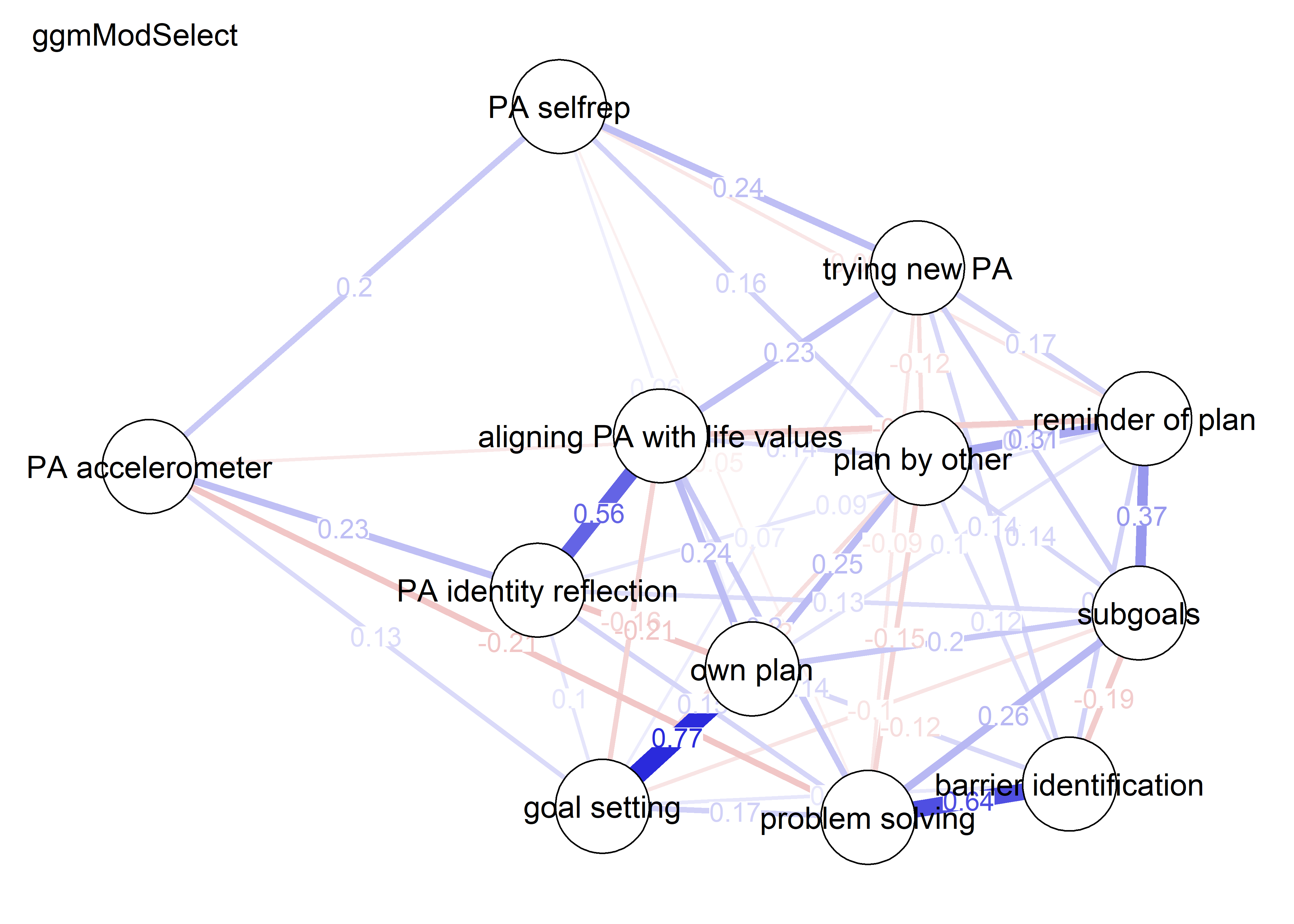
Centrality and stability
For interpretation, see:
Epskamp, S., Borsboom, D., & Fried, E. I. (2018). Estimating psychological networks and their accuracy: A tutorial paper. Behavior Research Methods, 50(1), 195-212. https://doi.org/10.3758/s13428-017-0862-1
For caveats to interpreting centrality, see:
Bringmann, L. F., Elmer, T., Epskamp, S., Krause, R. W., Schoch, D., Wichers, M., & Bringmann, L. What do centrality measures measure in psychological networks? Preprint available: https://www.researchgate.net/publication/329129039_What_do_centrality_measures_measure_in_psychological_networks
Hallquist, M., Wright, A. G. C., & Molenaar, P. C. M. (2019). Problems with centrality measures in psychopathology symptom networks: Why network psychometrics cannot escape psychometric theory. https://doi.org/10.31234/osf.io/pg4mf
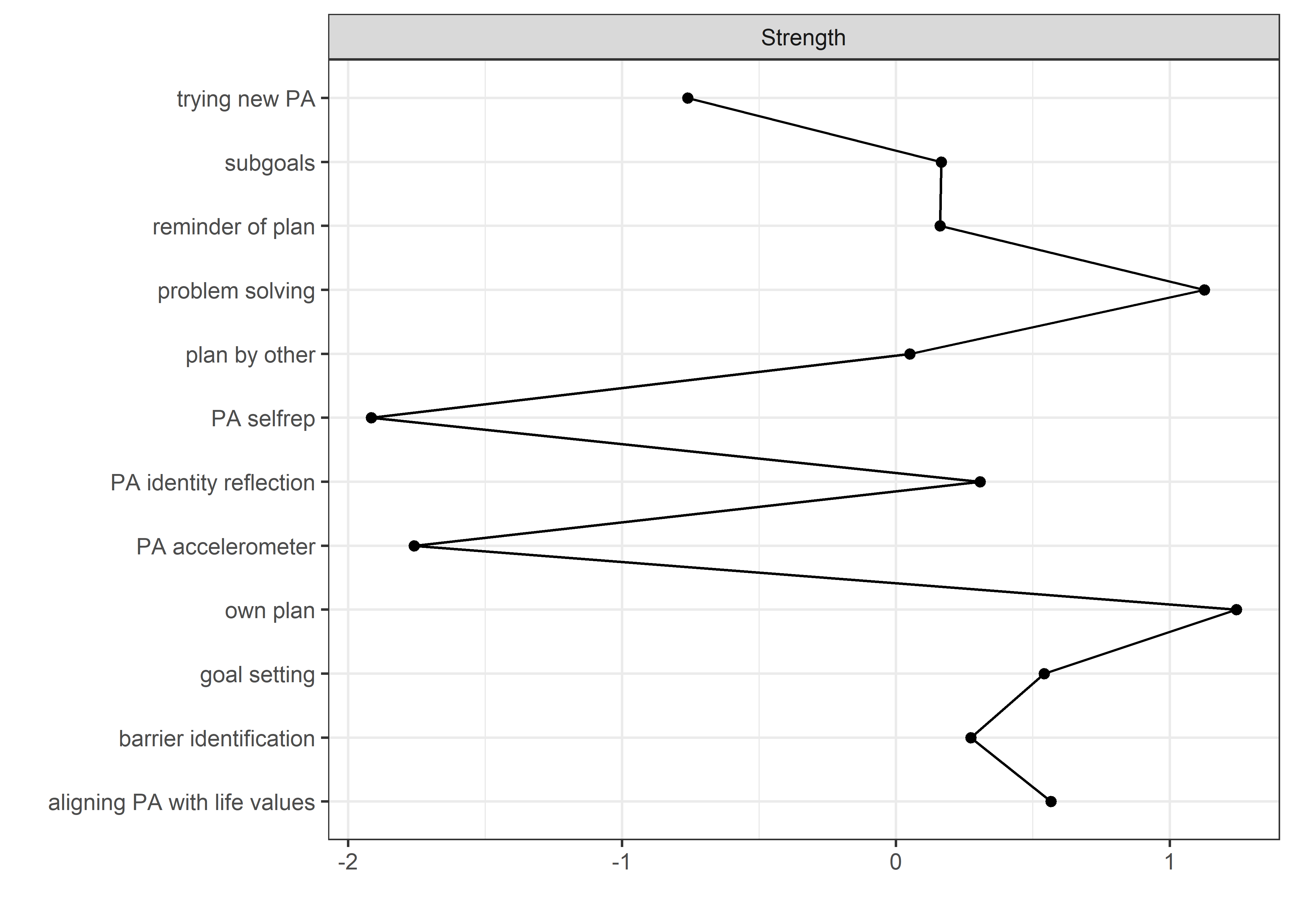
qgraph::centralityPlot(bootnetgraph,
               include = c("Strength", "ExpectedInfluence"),
               orderBy = "ExpectedInfluence")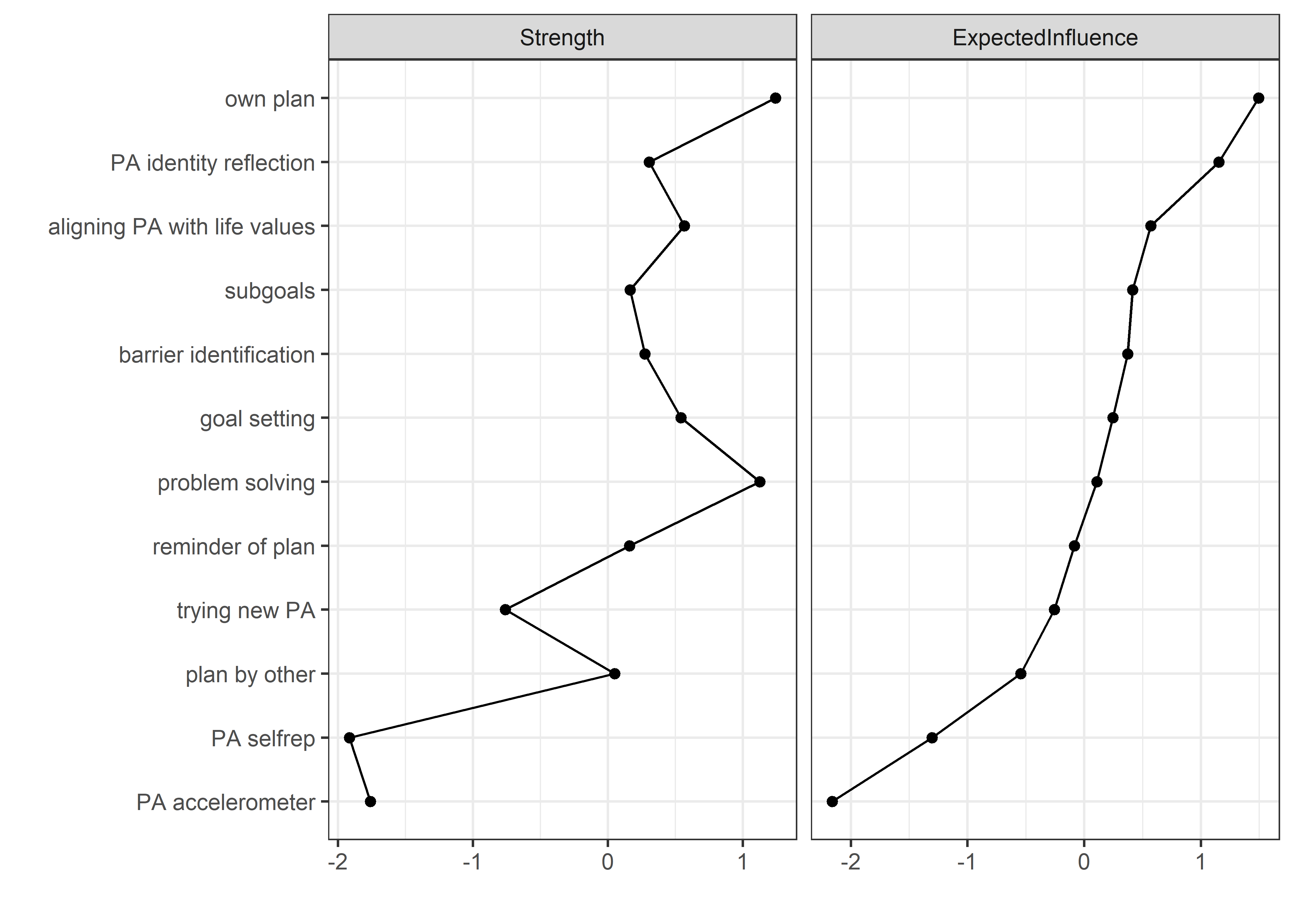
qgraph::centrality(bootnetgraph)$InDegree
##                   PA selfrep             PA accelerometer
##                    0.7975174                    0.8547198
##                 goal setting                     own plan
##                    1.7005088                    1.9586245
##                plan by other             reminder of plan
##                    1.5201372                    1.5606376
##                     subgoals                trying new PA
##                    1.5624020                    1.2218968
##       barrier identification              problem solving
##                    1.6020024                    1.9153104
##       PA identity reflection aligning PA with life values
##                    1.6144283                    1.7095057
scale(qgraph::centrality(bootnetgraph)$InDegree)
##                                     [,1]
## PA selfrep                   -1.91555770
## PA accelerometer             -1.75990258
## goal setting                  0.54159878
## own plan                      1.24396491
## plan by other                 0.05078431
## reminder of plan              0.16099129
## subgoals                      0.16579237
## trying new PA                -0.76076641
## barrier identification        0.27355011
## problem solving               1.12610179
## PA identity reflection        0.30736266
## aligning PA with life values  0.56608046
## attr(,"scaled:center")
## [1] 1.501474
## attr(,"scaled:scale")
## [1] 0.3674945
qgraph::centrality(bootnetgraph)$Closeness
##                   PA selfrep             PA accelerometer
##                   0.01043680                   0.01182721
##                 goal setting                     own plan
##                   0.01327433                   0.01443238
##                plan by other             reminder of plan
##                   0.01329430                   0.01324395
##                     subgoals                trying new PA
##                   0.01438012                   0.01268867
##       barrier identification              problem solving
##                   0.01324759                   0.01495958
##       PA identity reflection aligning PA with life values
##                   0.01421743                   0.01587286
qgraph::centrality(bootnetgraph)$Betweenness
##                   PA selfrep             PA accelerometer
##                            4                            4
##                 goal setting                     own plan
##                            4                           16
##                plan by other             reminder of plan
##                           10                            4
##                     subgoals                trying new PA
##                            4                            6
##       barrier identification              problem solving
##                            2                           12
##       PA identity reflection aligning PA with life values
##                            2                            8

cor(qgraph::centrality(bootnetgraph)$InDegree, qgraph::centrality(bootnetgraph)$Betweenness,
    method = "spearman")
## [1] 0.3596079

# bootnet_stability_individualAgreementBcts <- bootnet::bootnet(individualAgreementBCTs, stepwise = FALSE, nBoots=1000)
# save(bootnet_stability_individualAgreementBcts, file = "./Rdata_files/bootnet_stability_individualAgreementBcts.Rdata")
load("./Rdata_files/bootnet_stability_individualAgreementBcts.Rdata")

plot(bootnet_stability_individualAgreementBcts, labels = TRUE, order = "sample") 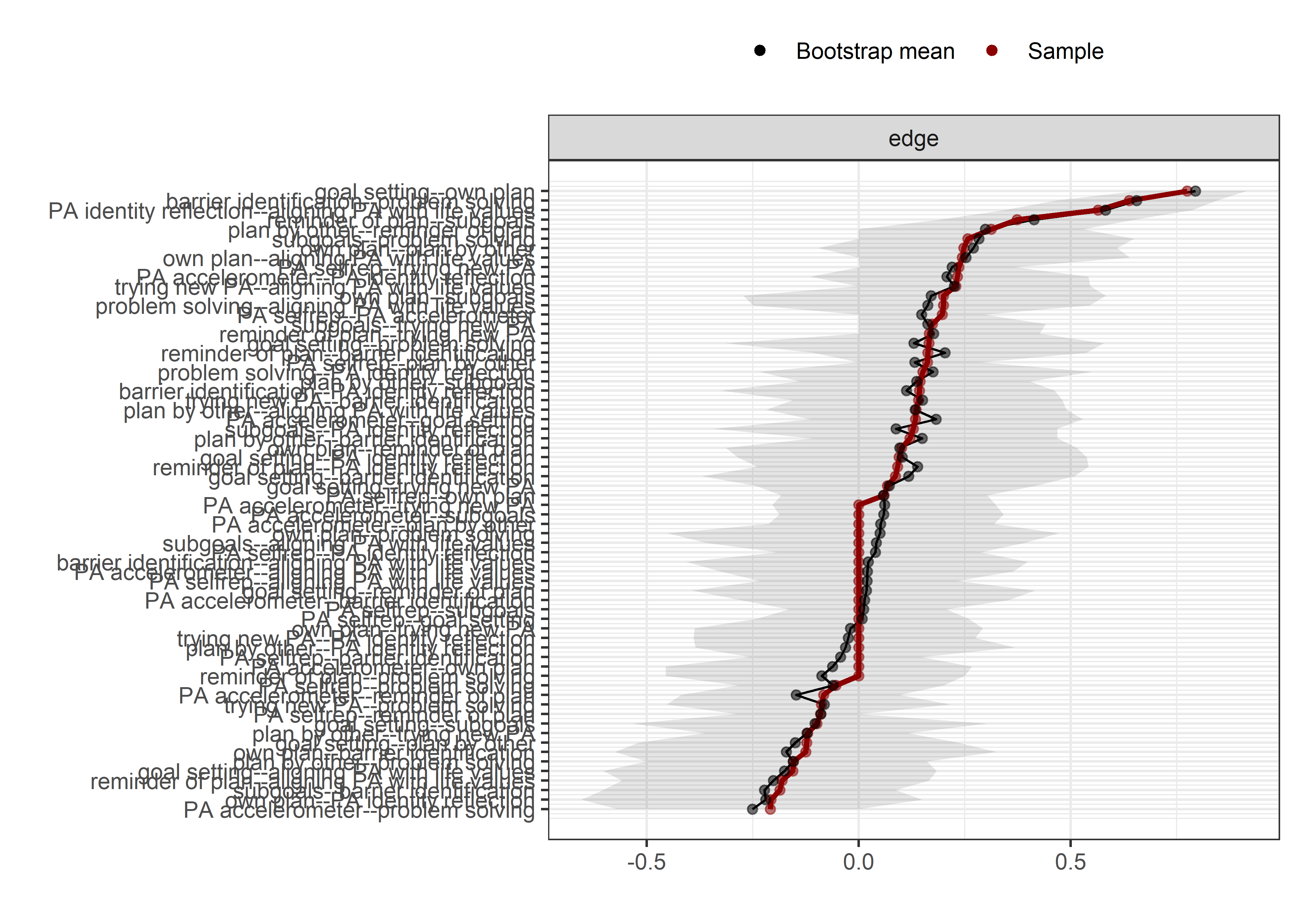
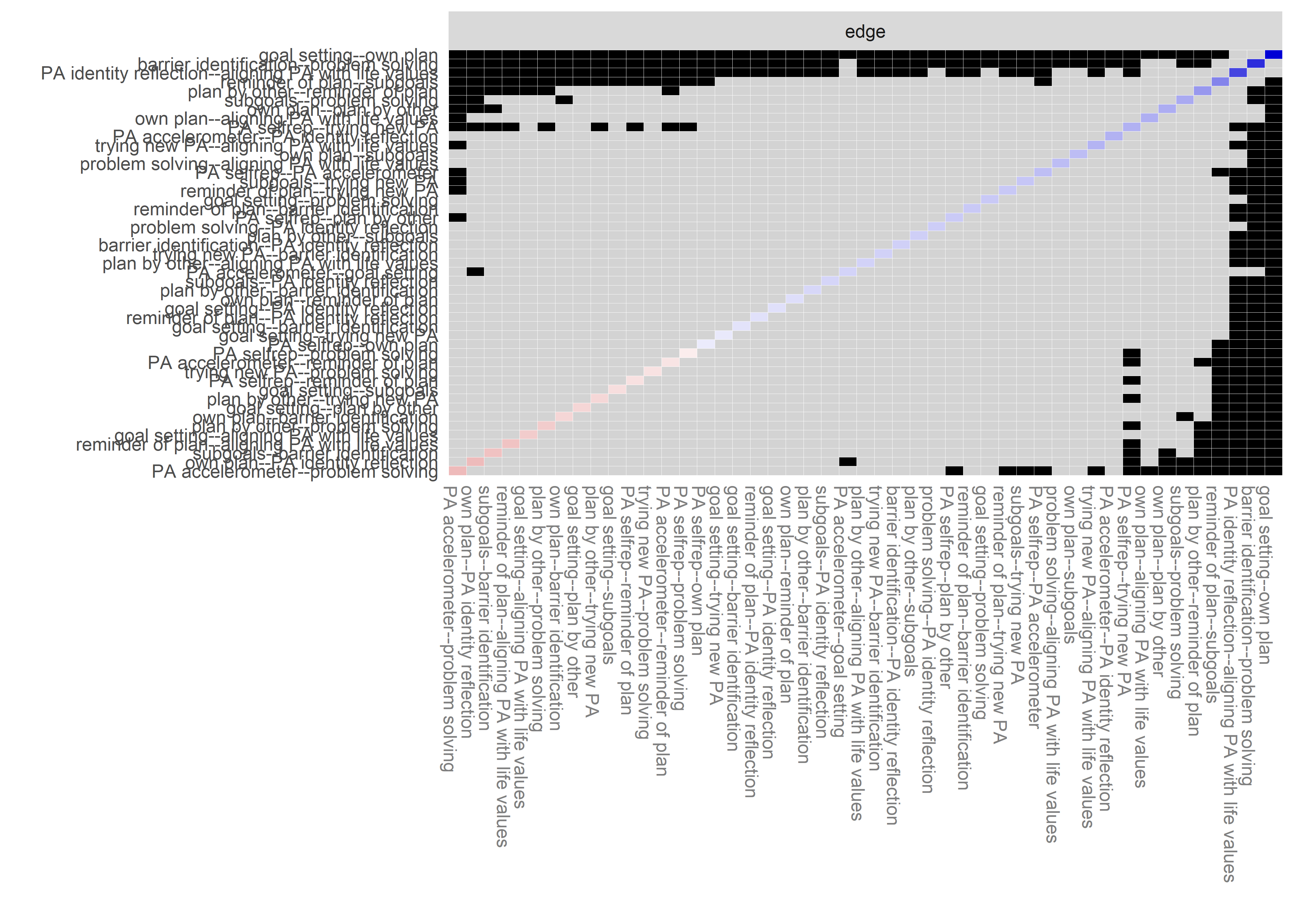
# # Failed to run
# bootnet_centrality_stability_individualAgreementBcts <- bootnet::bootnet(individualAgreementBCTs, stepwise = FALSE, nBoots=1000, type="case")
# save(bootnet_centrality_stability_individualAgreementBcts, file = "./Rdata_files/bootnet_centrality_stability_individualAgreementBcts.Rdata")
# load("./Rdata_files/bootnet_centrality_stability_individualAgreementBcts.Rdata")
#
# plot(bootnet_centrality_stability_individualAgreementBcts)
# plot(bootnet_centrality_stability_individualAgreementBcts, perNode=T, "strength")
#
# bootnet::corStability(bootnet_centrality_stability_individualAgreementBcts)
Combined agreement-related BCTs and PA
bctdf_pa_combinedAgreementBcts <- df %>% dplyr::select(
  'PA selfrep' = padaysLastweek_T1,
  'PA accelerometer' = mvpaAccelerometer_T1,
  'goal setting' = PA_agreementDependentBCT_01_T1,
  'own plan' = PA_agreementDependentBCT_02_T1,
  'plan by other' = PA_agreementDependentBCT_03_T1,
  'reminder of plan' = PA_agreementDependentBCT_04_T1,
  'subgoals' = PA_agreementDependentBCT_05_T1,
  'trying new PA' = PA_agreementDependentBCT_06_T1,
  'barrier identification' = PA_agreementDependentBCT_07_T1,
  'problem solving' = PA_agreementDependentBCT_08_T1,
  'PA identity reflection' = PA_agreementDependentBCT_09_T1,
  'aligning PA with life values' = PA_agreementDependentBCT_10_T1) %>%
 rowwise() %>%
 mutate(
  'goal setting' = ifelse(`goal setting` == 1, 0, 1),
  'has plan' = ifelse(`own plan` == 1 & `plan by other` == 1, 0, 1),
  # 'own plan' = ifelse(`own plan` == 1, 0, 1),
  'reminder of plan' = ifelse(`reminder of plan` == 1, 0, 1),
  'subgoals' = ifelse(`subgoals` == 1, 0, 1),
  'trying new PA' = ifelse(`trying new PA` == 1, 0, 1),
  # 'plan by other' = ifelse(`plan by other` == 1, 0, 1),
  # 'barrier identification' = ifelse(`barrier identification` == 1, 0, 1),
  # 'problem solving' = ifelse(`problem solving` == 1, 0, 1),
  'barriers identified or planned for' = ifelse(`problem solving` == 1 & `barrier identification` == 1, 0, 1),
  # 'PA identity reflection' = ifelse(`PA identity reflection` == 1, 0, 1),
  # 'aligning PA with life values' = ifelse(`aligning PA with life values` == 1, 0, 1)) %>%
  'identity, life values' = ifelse(`PA identity reflection` == 1 & `aligning PA with life values` == 1, 0, 1)) %>%
  dplyr::select(-`plan by other`, -`own plan`,
         -`barrier identification`, -`problem solving`, # closely related
         -`PA identity reflection`, -`aligning PA with life values`) %>% # closely related
  mutate_all(as.numeric)
mgm estimation
# devtools::install_github("jmbh/mgm")
# Restart R for the latest package
# .r.restartR()

# mgm wants full data, see package missForest for imputation
bctdf_pa_combinedAgreementBcts <- bctdf_pa_combinedAgreementBcts %>% na.omit()
# bctdf_pa_combinedAgreementBcts %>% names()
mgm_pa_variable_types <- c("g", "g", rep("c", 7))
mgm_pa_variable_levels <- c("1", "1", rep("2", 7))
# data.frame(mgm_pa_variable_types, mgm_pa_variable_levels, names(bctdf_pa_combinedAgreementBcts))

mgm_obj <- mgm::mgm(data = bctdf_pa_combinedAgreementBcts,
  type = mgm_pa_variable_types,
  level = mgm_pa_variable_levels,
  lambdaSel = "CV",
  lambdaFolds = 10,
  pbar = FALSE,
  binarySign = TRUE)
## Note that the sign of parameter estimates is stored separately; see ?mgm

pred_obj <- predict(object = mgm_obj,
                         data = bctdf_pa_combinedAgreementBcts)

pred_obj$errors
# Take R2 from gaussian, CC from categorical variables
pie_errors <- c(pred_obj$errors[1, 3],
                pred_obj$errors[2, 3],
                pred_obj$errors[3:nrow(pred_obj$errors), 4])

# PLOT NETWORK

node_colors <- c(viridis::viridis(4, begin = 0.3, end = 0.8)[1],
                 viridis::viridis(4, begin = 0.3, end = 0.8)[2],
                 rep(viridis::viridis(4, begin = 0.3, end = 0.8)[3], 7))

BCT_mgm <- qgraph::qgraph(mgm_obj$pairwise$wadj,
            layout = "spring",
            repulsion = 1, # To nudge the network from originally bad visual state
            title = "agreement-measured BCTs and PA",
            edge.color = ifelse(mgm_obj$pairwise$edgecolor == "darkgreen", "blue", mgm_obj$pairwise$edgecolor),
            pie = pie_errors,
            pieColor = viridis::viridis(4, begin = 0.3, end = 0.8)[4],
            color = node_colors,
            labels = names(bctdf_pa_combinedAgreementBcts),
            label.cex = 0.75,
            label.scale = FALSE,
            label.color = c(rep("black", 9)))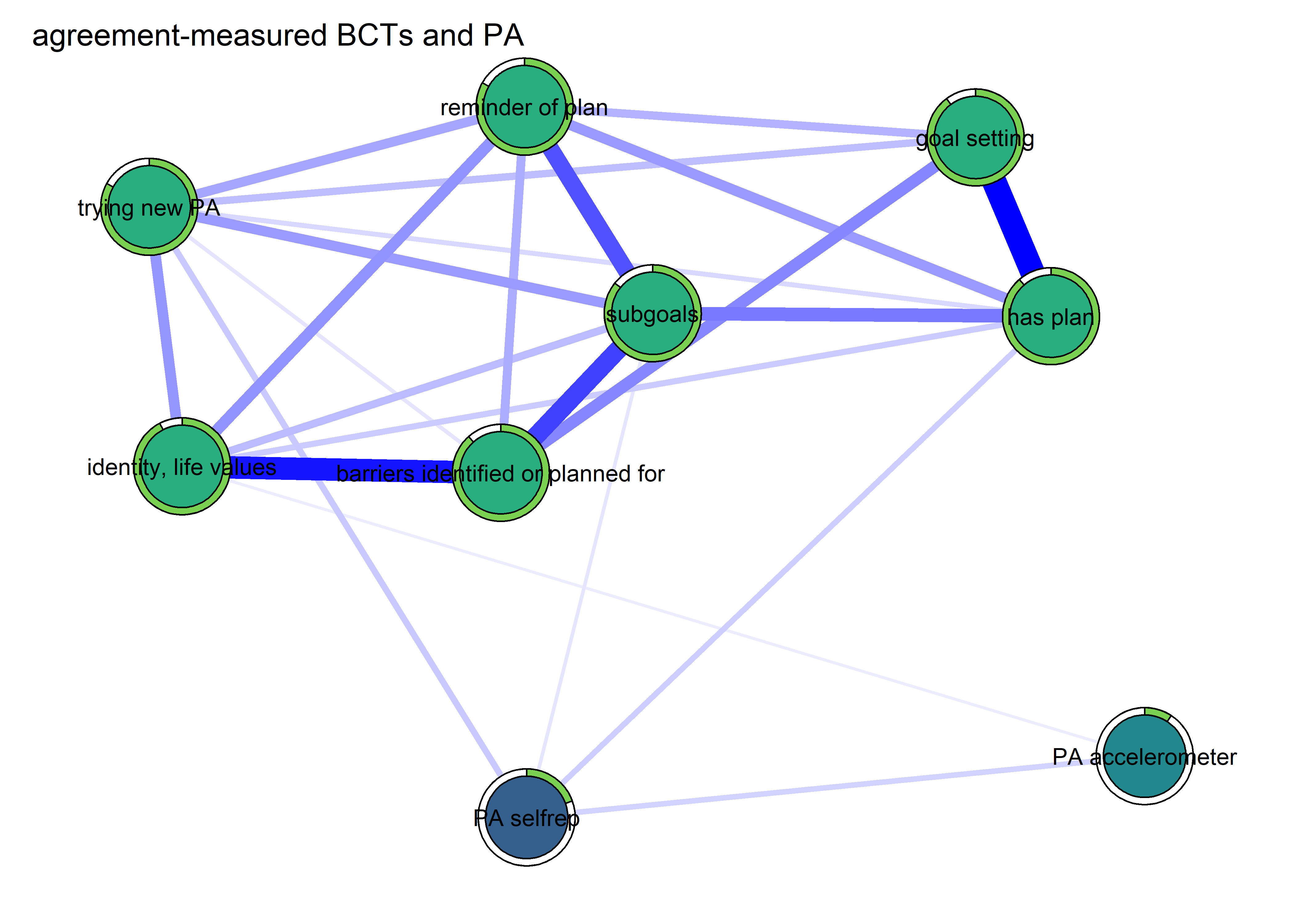
GGM plot
combinedAgreementBcts_ggm_df <- df %>% dplyr::select(
  'PA selfrep' = padaysLastweek_T1,
  'PA accelerometer' = mvpaAccelerometer_T1,
  'goal setting' = PA_agreementDependentBCT_01_T1,
  'own plan' = PA_agreementDependentBCT_02_T1,
  'plan by other' = PA_agreementDependentBCT_03_T1,
  'reminder of plan' = PA_agreementDependentBCT_04_T1,
  'subgoals' = PA_agreementDependentBCT_05_T1,
  'trying new PA' = PA_agreementDependentBCT_06_T1,
  'barrier identification' = PA_agreementDependentBCT_07_T1,
  'problem solving' = PA_agreementDependentBCT_08_T1,
  'PA identity reflection' = PA_agreementDependentBCT_09_T1,
  'aligning PA with life values' = PA_agreementDependentBCT_10_T1) %>%
 rowwise() %>%
 mutate(
  'has plan' = mean(c(`own plan`, `plan by other`), na.rm = TRUE),
  'barriers identified or planned for' = mean(c(`problem solving`, `barrier identification`), na.rm = TRUE),
  'identity, life values' = mean(c(`PA identity reflection` == 1, `aligning PA with life values`), na.rm = TRUE)) %>%
  dplyr::select(-`plan by other`, -`own plan`,
         -`barrier identification`, -`problem solving`, # closely related
         -`PA identity reflection`, -`aligning PA with life values`) %>% # closely related
  mutate_all(as.numeric)

# Create means for filling nodes
# piefill_ggm <- S.total_ggm %>%
#   dplyr::select(-contains("MVPA"), -girl, -intervention) %>%
#   summarise_all(funs(median(., na.rm = TRUE) / 6))
#
# piefill_ggm$MVPA <- median(S.total_ggm$MVPA, na.rm = TRUE) / (60*24)
# piefill_ggm$girl <- mean(S.total_ggm$girl, na.rm = TRUE)
# piefill_ggm$intervention <- mean(S.total_ggm$intervention, na.rm = TRUE)
#
# piefill_ggm <- piefill_ggm %>% dplyr::select(MVPA, girl, intervention, everything())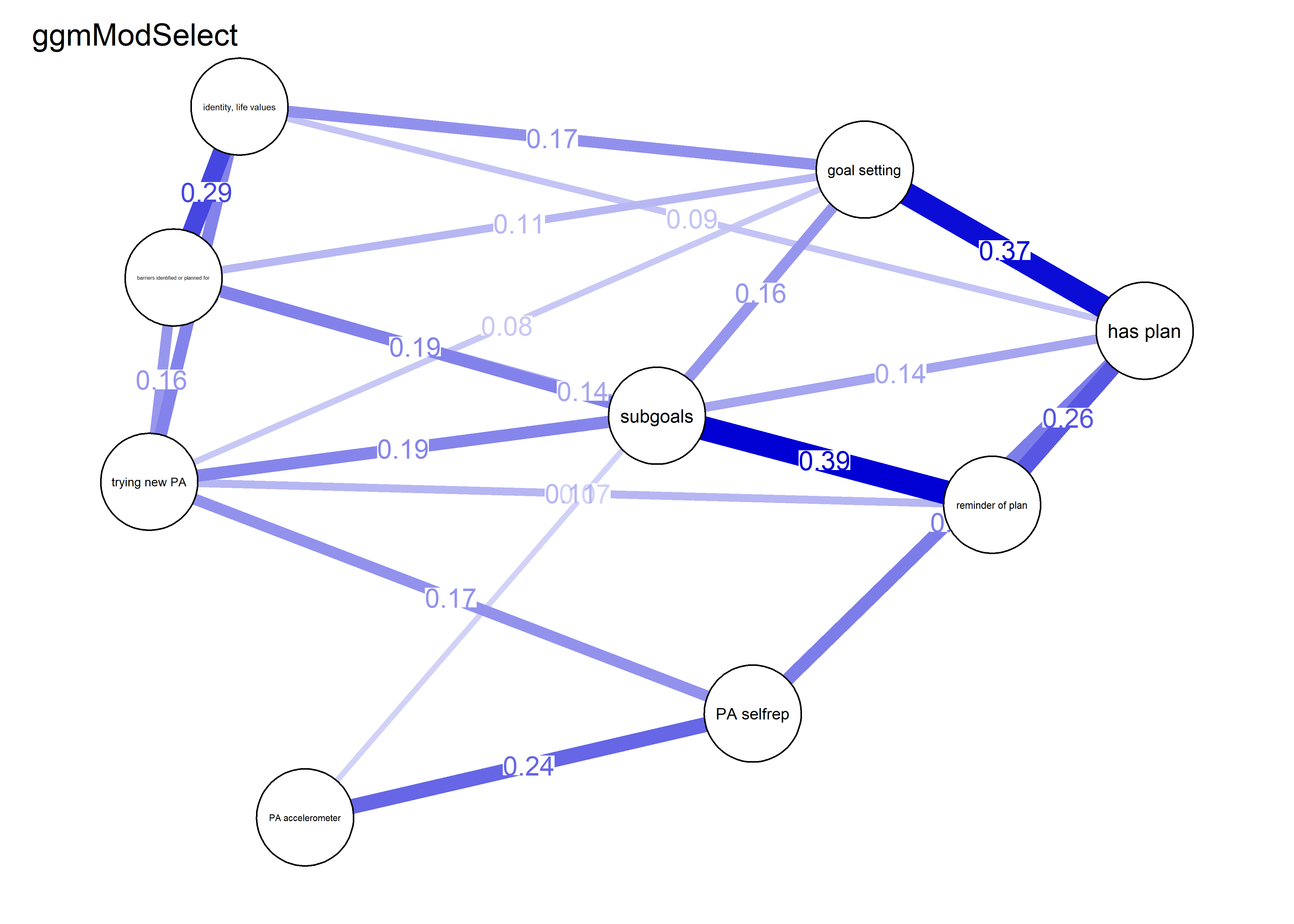
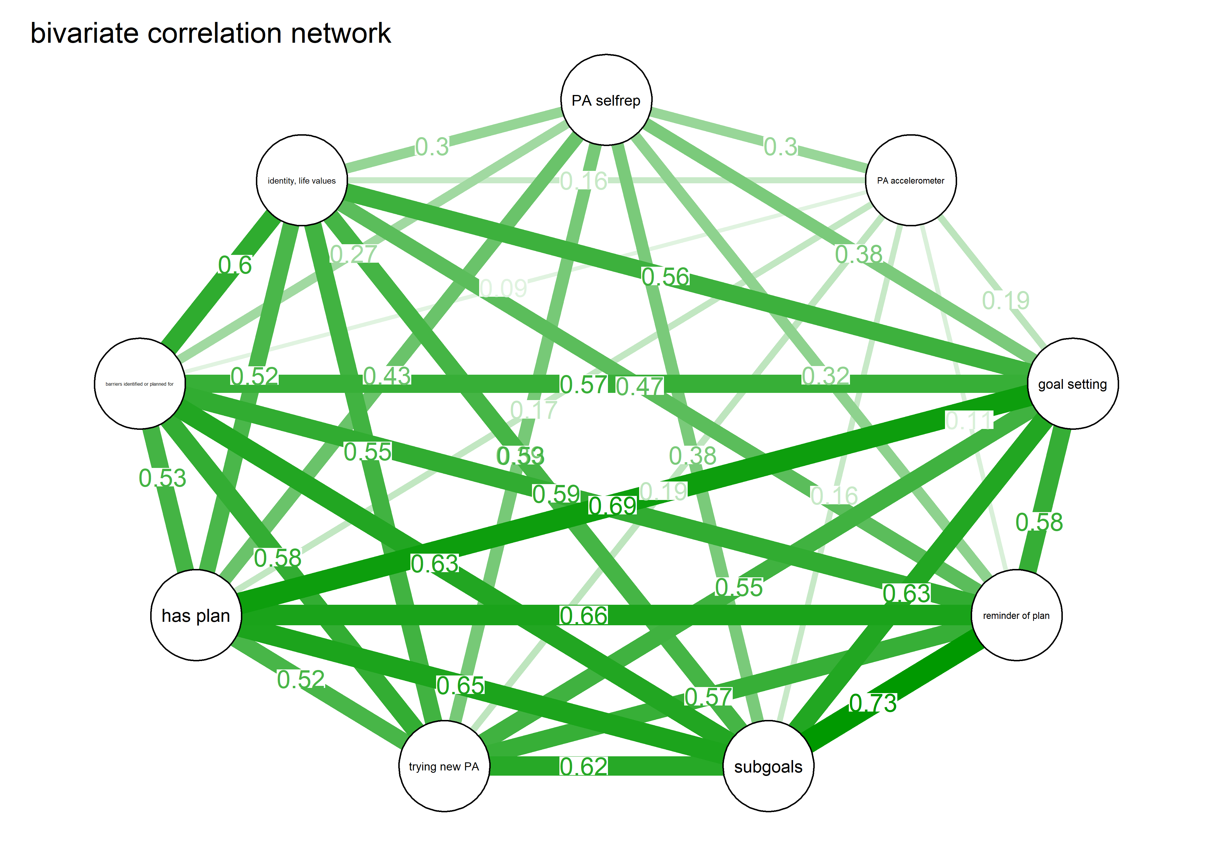
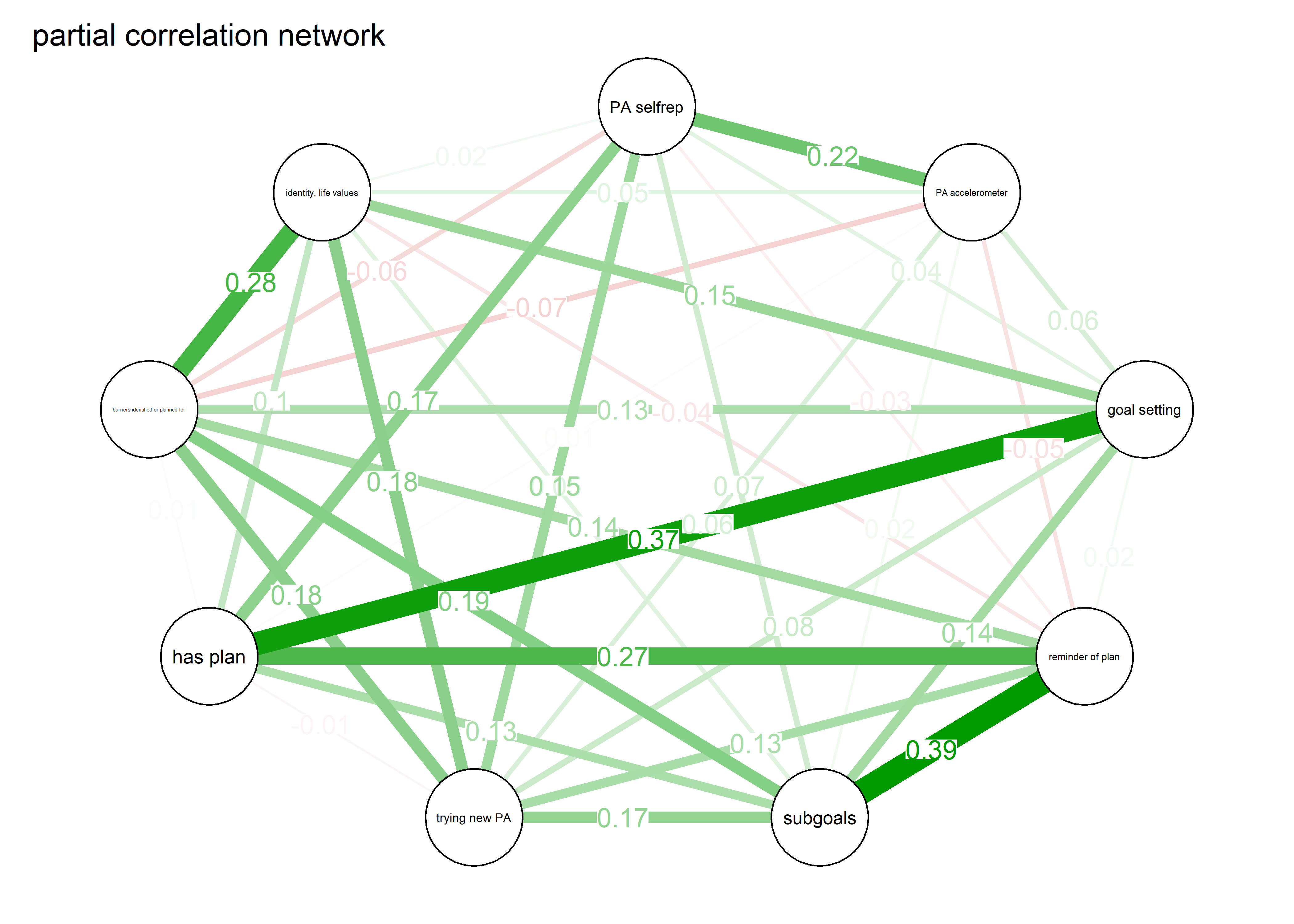
# Average the layout of three previous plots, and plot each according to that
avlayout <- qgraph::averageLayout(bootnetgraph, corgraph, pcorgraph)

corgraph <- qgraph::qgraph(qgraph::cor_auto(combinedAgreementBcts_ggm_df), graph = "cor",
       labels = names(combinedAgreementBcts_ggm_df),
       edge.labels = TRUE,
       layout = avlayout,
       title = "bivariate correlation network",
       theme = "colorblind",
       maximum = max(c(bootnetgraph$graph$Graph$maximum,
                     pcorgraph$graph$Graph$maximum,
                     corgraph$graph$Graph$maximum)),
       label.scale = FALSE)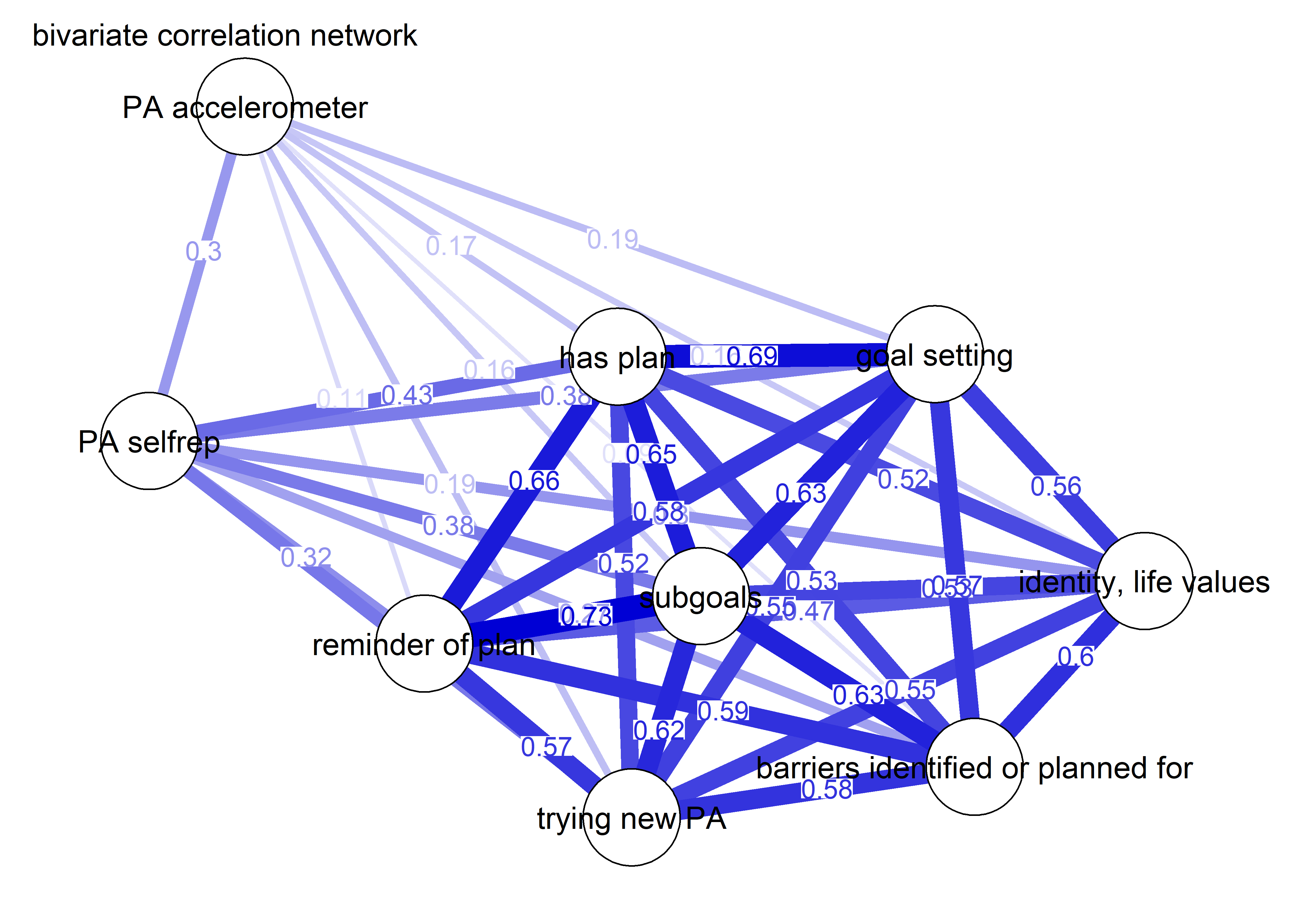
# To help with visual comparison, that last argument takes the maximum edge of the three
# graphs and places that as the benchmark for the thickest line in all plots.

pcorgraph <- qgraph::qgraph(qgraph::cor_auto(combinedAgreementBcts_ggm_df), graph = "pcor",
       labels = names(combinedAgreementBcts_ggm_df),
       edge.labels = TRUE,
       layout = avlayout,
       title = "partial correlation network",
       theme = "colorblind",
       maximum = max(c(bootnetgraph$graph$Graph$maximum,
                     pcorgraph$graph$Graph$maximum,
                     corgraph$graph$Graph$maximum)),
       label.scale = FALSE)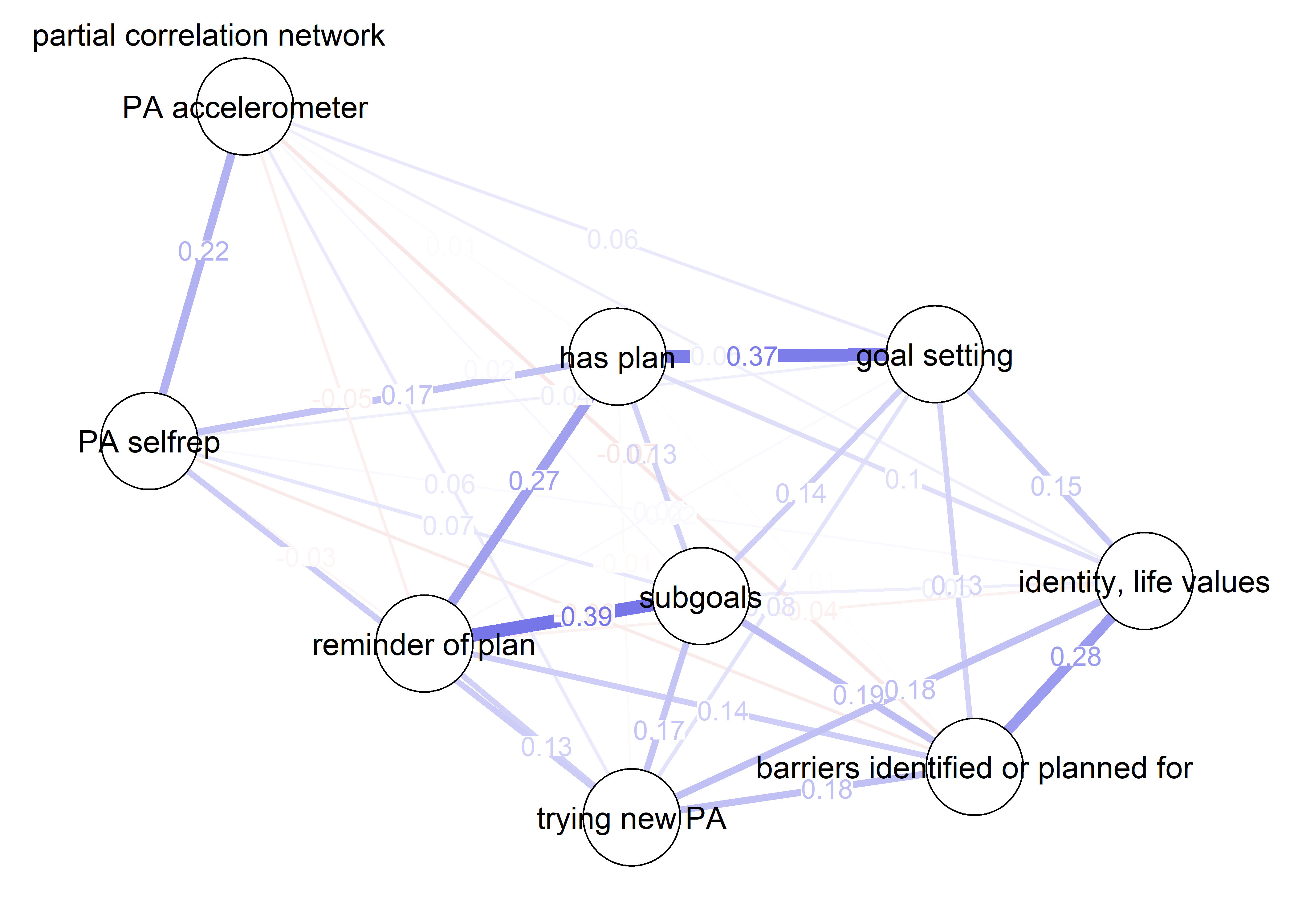
bootnetgraph <- plot(combinedAgreementBcts_network,
                     edge.labels = TRUE,
                     layout = avlayout,
                     title = "ggmModSelect",
       maximum = max(c(bootnetgraph$graph$Graph$maximum,
                     pcorgraph$graph$Graph$maximum,
                     corgraph$graph$Graph$maximum)),
       label.scale = FALSE)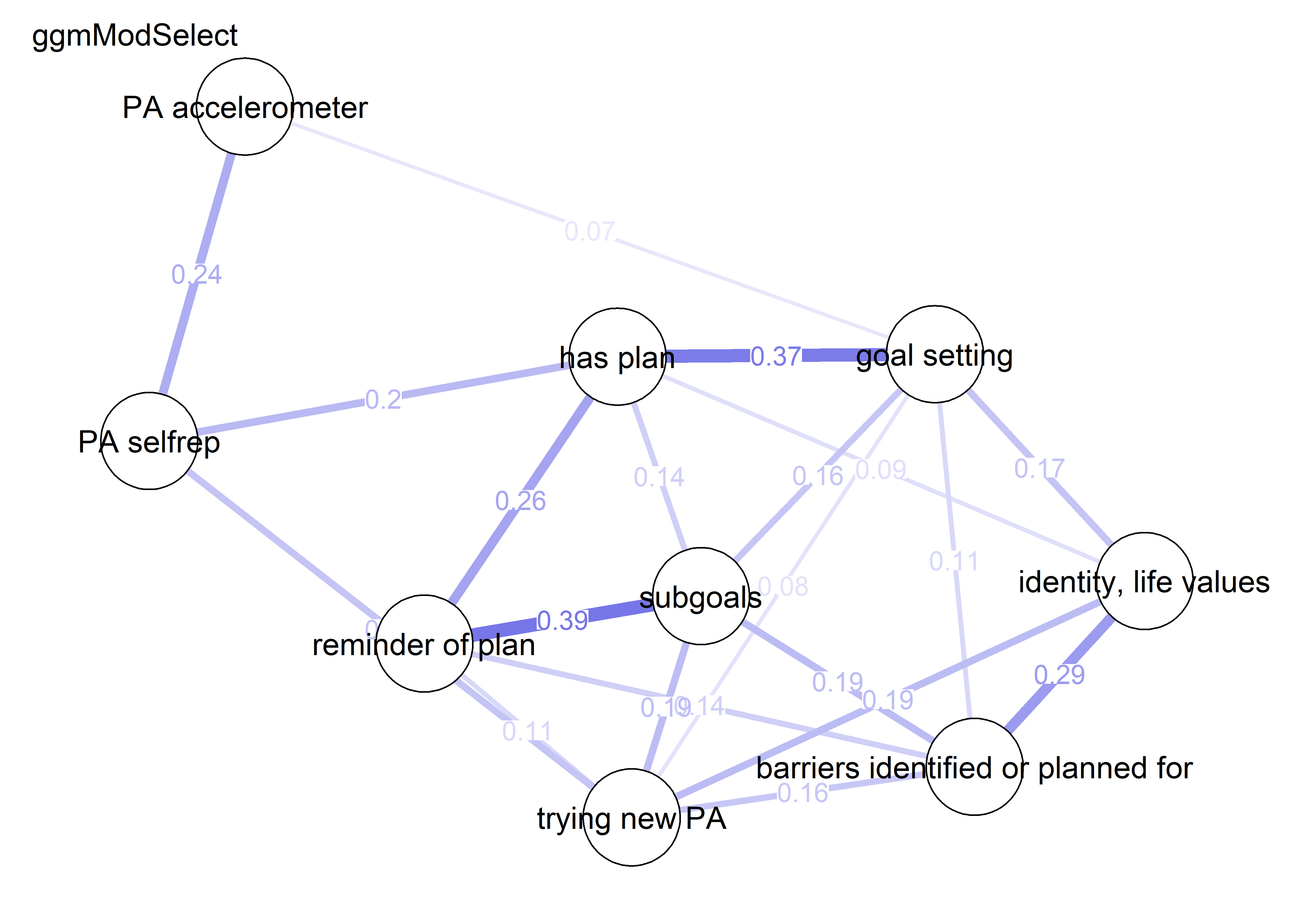
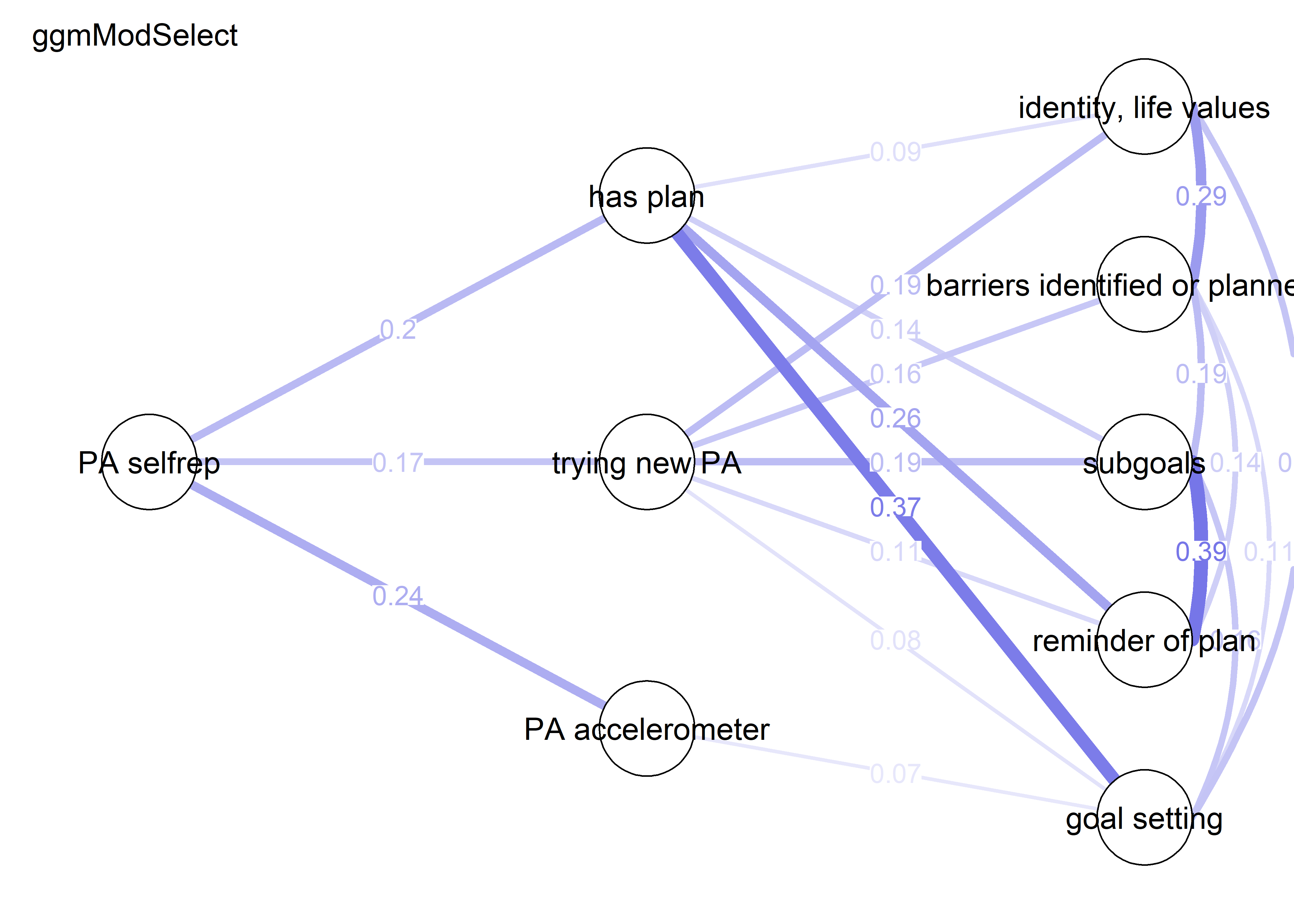
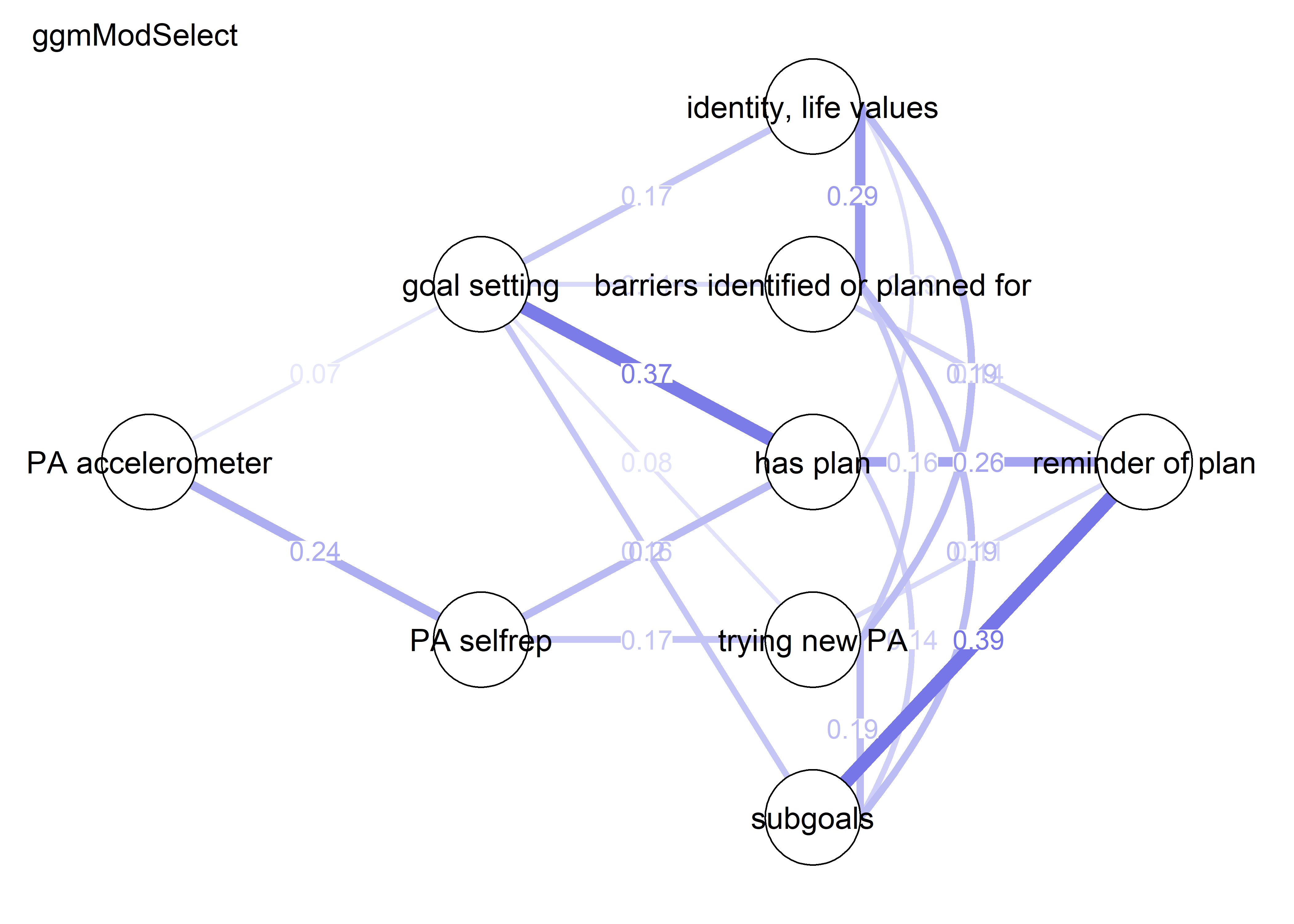
Centrality and stability
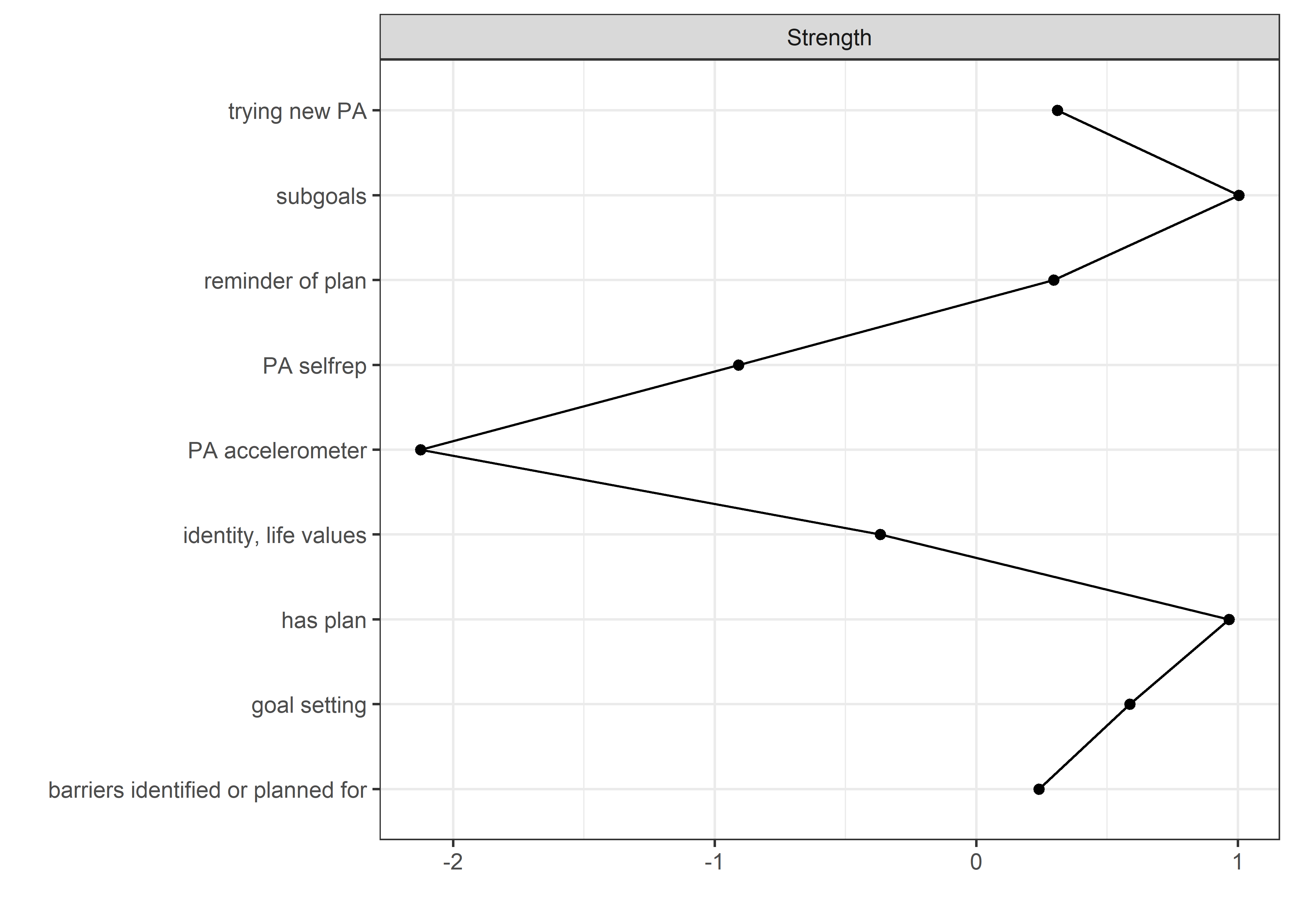
qgraph::centralityPlot(bootnetgraph,
               include = c("Strength", "ExpectedInfluence"),
               orderBy = "ExpectedInfluence")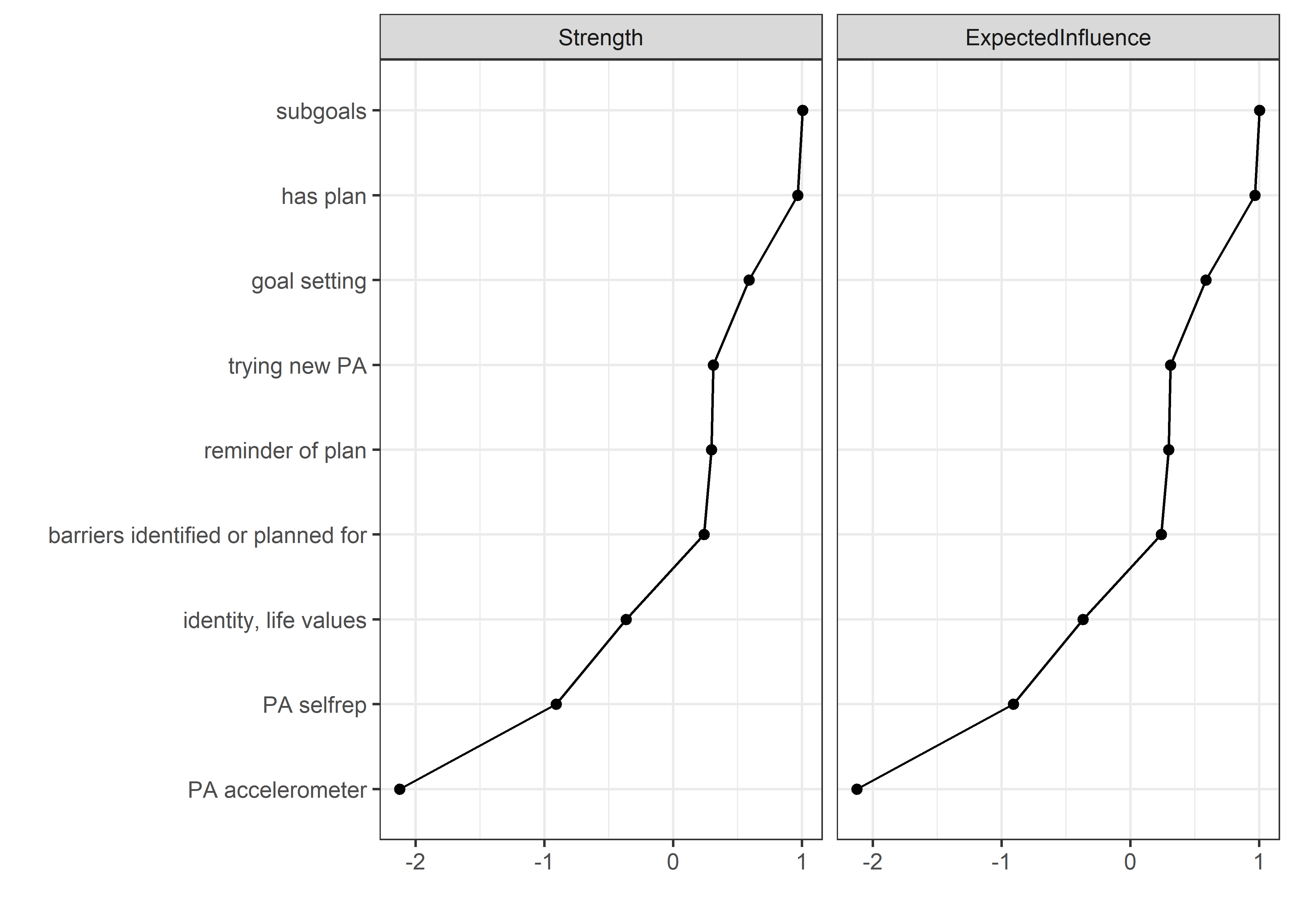
qgraph::centrality(bootnetgraph)$InDegree
##                         PA selfrep                   PA accelerometer
##                          0.6041888                          0.3051056
##                       goal setting                   reminder of plan
##                          0.9724035                          0.9009387
##                           subgoals                      trying new PA
##                          1.0750300                          0.9042554
##                           has plan barriers identified or planned for
##                          1.0657890                          0.8869149
##              identity, life values
##                          0.7375737
scale(qgraph::centrality(bootnetgraph)$InDegree)
##                                          [,1]
## PA selfrep                         -0.9093427
## PA accelerometer                   -2.1243949
## goal setting                        0.5865619
## reminder of plan                    0.2962297
## subgoals                            1.0034912
## trying new PA                       0.3097042
## has plan                            0.9659489
## barriers identified or planned for  0.2392569
## identity, life values              -0.3674551
## attr(,"scaled:center")
## [1] 0.8280222
## attr(,"scaled:scale")
## [1] 0.2461485
qgraph::centrality(bootnetgraph)$Closeness
##                         PA selfrep                   PA accelerometer
##                         0.01487797                         0.01031179
##                       goal setting                   reminder of plan
##                         0.01622229                         0.01641658
##                           subgoals                      trying new PA
##                         0.01616400                         0.01573626
##                           has plan barriers identified or planned for
##                         0.01692116                         0.01409724
##              identity, life values
##                         0.01441236
qgraph::centrality(bootnetgraph)$Betweenness
##                         PA selfrep                   PA accelerometer
##                                 16                                  0
##                       goal setting                   reminder of plan
##                                  2                                  4
##                           subgoals                      trying new PA
##                                  2                                 12
##                           has plan barriers identified or planned for
##                                 10                                  4
##              identity, life values
##                                  2

cor(qgraph::centrality(bootnetgraph)$InDegree, qgraph::centrality(bootnetgraph)$Betweenness,
    method = "spearman")
## [1] 0.07661309

# bootnet_stability_combinedAgreementBcts <- bootnet::bootnet(combinedAgreementBcts_network, stepwise = FALSE, nBoots=1000)
# save(bootnet_stability_combinedAgreementBcts, file = "./Rdata_files/bootnet_stability_combinedAgreementBcts.Rdata")
load("./Rdata_files/bootnet_stability_combinedAgreementBcts.Rdata")

plot(bootnet_stability_combinedAgreementBcts, labels = TRUE, order = "sample") 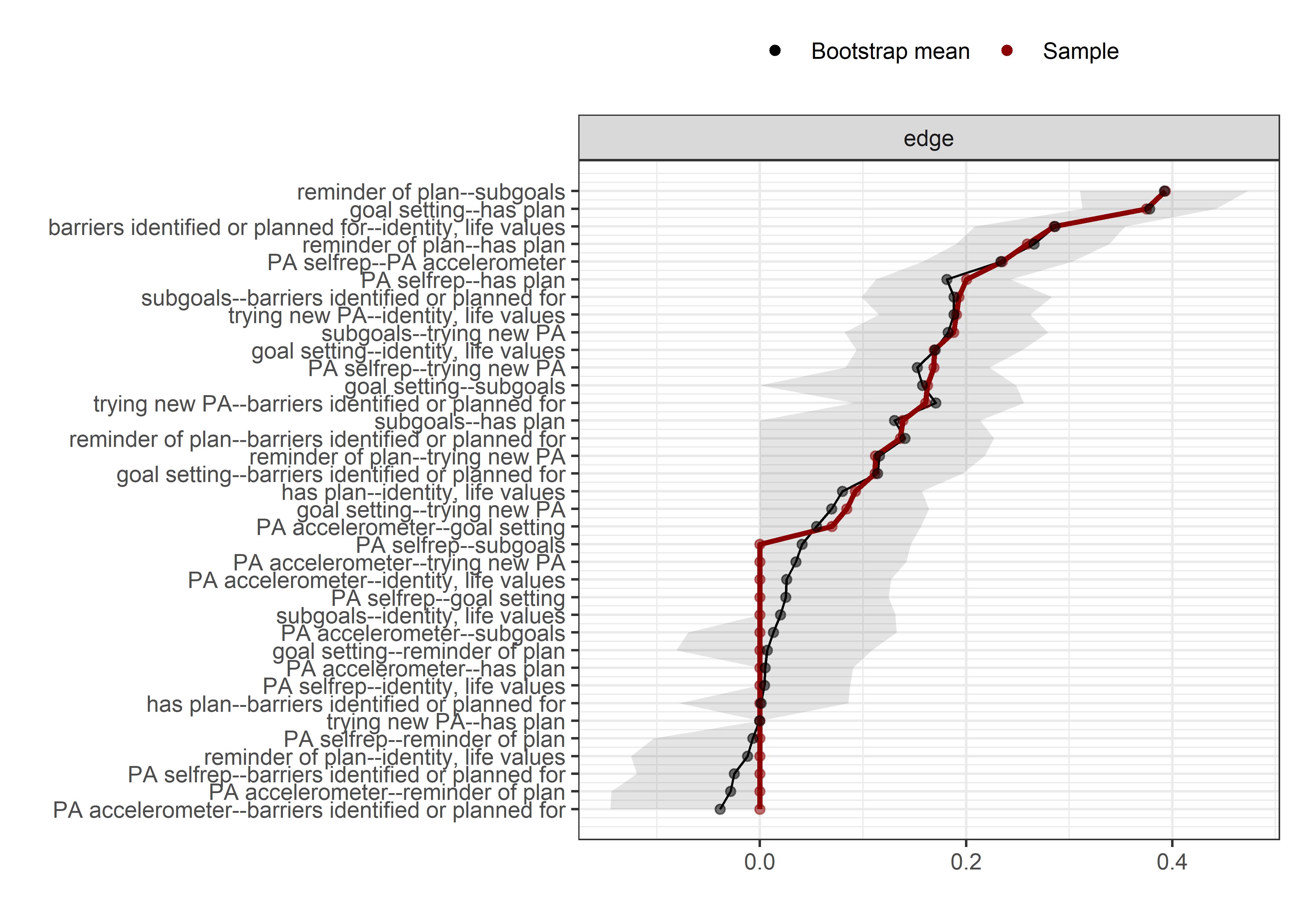
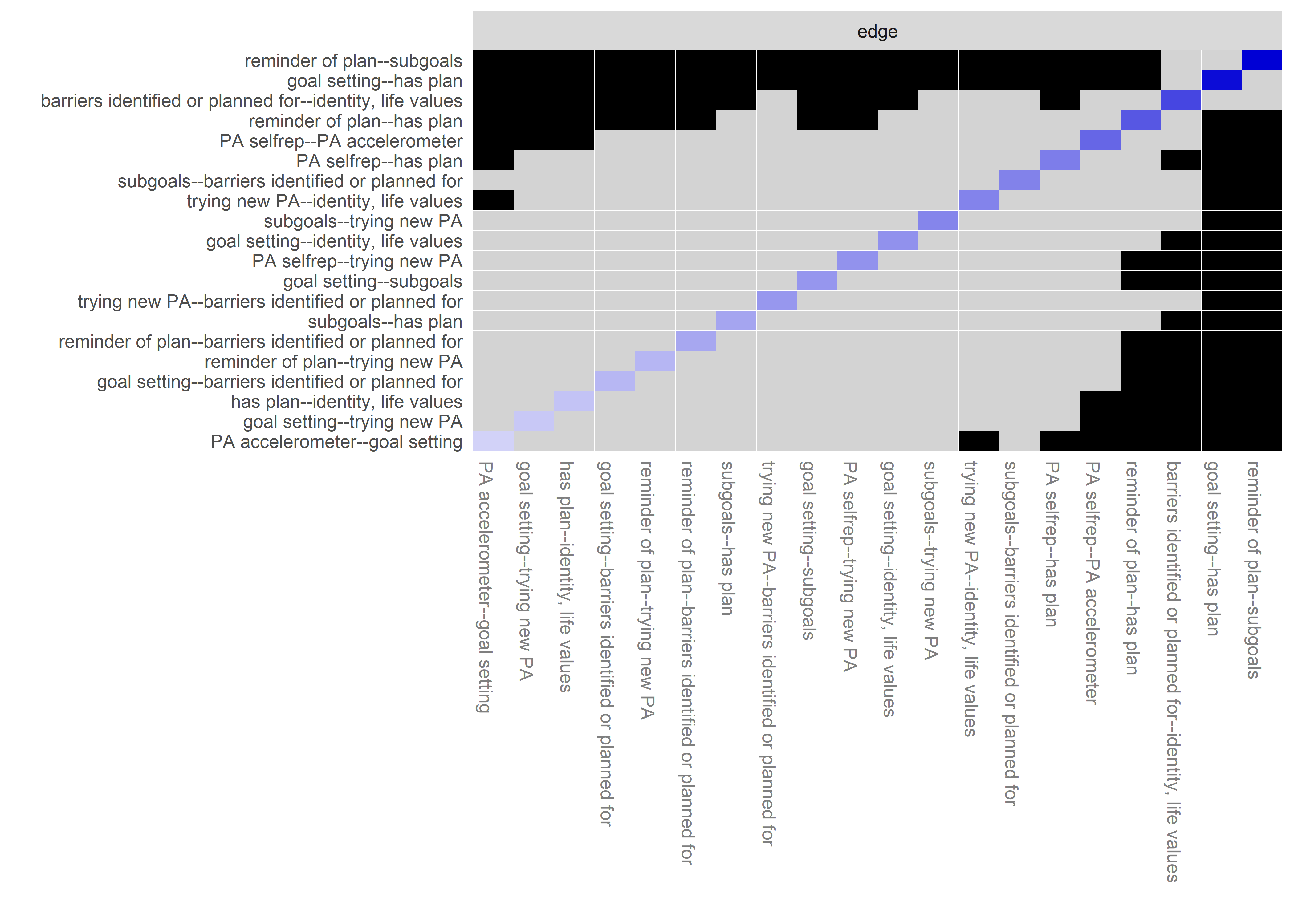
# bootnet_centrality_stability_combinedAgreementBcts <- bootnet::bootnet(combinedAgreementBcts_network, stepwise = FALSE, nBoots=1000,nCores=8, type="case")
# save(bootnet_centrality_stability_combinedAgreementBcts, file = "./Rdata_files/bootnet_centrality_stability_combinedAgreementBcts.Rdata")
# load("./Rdata_files/bootnet_centrality_stability_combinedAgreementBcts.Rdata")
#
# plot(bootnet_centrality_stability_combinedAgreementBcts)
# plot(bootnet_centrality_stability_combinedAgreementBcts, perNode=T, "strength")
#
# bootnet::corStability(bootnet_centrality_stability_combinedAgreementBcts)
Heterogeneity
The smallest track (IT) has 163 observations. According to the heuristic sample size for p variables for Gaussian data, (p*(p-1)/2 + p), we could estimate about 7 variables. (based on these slides referring to this source: BĂźhlmann, P. & van de Geer, S. (2011). Statistics for High-Dimensional Data: Methods, Theory and Applications. Springer.)
All tracks seem sufficiently similar on these BCTs.
combinedAgreementBcts_tracks_df <- df %>%
  dplyr::select(
  'PA selfrep' = padaysLastweek_T1,
  # 'PA accelerometer' = mvpaAccelerometer_T1,
  'Autonomous' = PA_autonomous_T1,
  'goal setting' = PA_agreementDependentBCT_01_T1,
  'own plan' = PA_agreementDependentBCT_02_T1,
  # 'plan by other' = PA_agreementDependentBCT_03_T1,
  'reminder of plan' = PA_agreementDependentBCT_04_T1,
  'subgoals' = PA_agreementDependentBCT_05_T1,
  # 'trying new PA' = PA_agreementDependentBCT_06_T1,
  'barrier identification' = PA_agreementDependentBCT_07_T1,
  'problem solving' = PA_agreementDependentBCT_08_T1,
  'PA identity reflection' = PA_agreementDependentBCT_09_T1,
  'aligning PA with life values' = PA_agreementDependentBCT_10_T1) %>%
 rowwise() %>%
 mutate(
  'barriers identified or planned for' = mean(c(`problem solving`, `barrier identification`), na.rm = TRUE),
  'identity, life values' = mean(c(`PA identity reflection` == 1, `aligning PA with life values`), na.rm = TRUE)) %>%
  dplyr::select(
         -`barrier identification`, -`problem solving`, # closely related
         -`PA identity reflection`, -`aligning PA with life values`) %>% # closely related
  mutate_all(as.numeric)

combinedAgreementBcts_tracks_df <- cbind(track = df$track, combinedAgreementBcts_tracks_df)

combinedAgreementBcts_tracks_df %>% dplyr::group_by(track) %>% summarise(n = n())
heterogeneity_Nur <- combinedAgreementBcts_tracks_df %>%
  dplyr::filter(track == "Nur") %>%
  na.omit() %>%
  dplyr::select(-track)

heterogeneity_HRC <- combinedAgreementBcts_tracks_df %>%
  dplyr::filter(track == "HRC") %>%
  na.omit() %>%
  dplyr::select(-track)

heterogeneity_BA <- combinedAgreementBcts_tracks_df %>%
  dplyr::filter(track == "BA") %>%
  na.omit() %>%
  dplyr::select(-track)

heterogeneity_IT <- combinedAgreementBcts_tracks_df %>%
  dplyr::filter(track == "IT") %>%
  na.omit() %>%
  dplyr::select(-track)

network_Nur <- bootnet::estimateNetwork(heterogeneity_Nur, default="ggmModSelect")
network_HRC <- bootnet::estimateNetwork(heterogeneity_HRC, default="ggmModSelect")
network_BA <- bootnet::estimateNetwork(heterogeneity_BA, default="ggmModSelect")
network_IT <- bootnet::estimateNetwork(heterogeneity_IT, default="ggmModSelect")

graph_Nur <- plot(network_Nur, layout="spring", cut=0, label.scale = FALSE, title = "Practical nurse")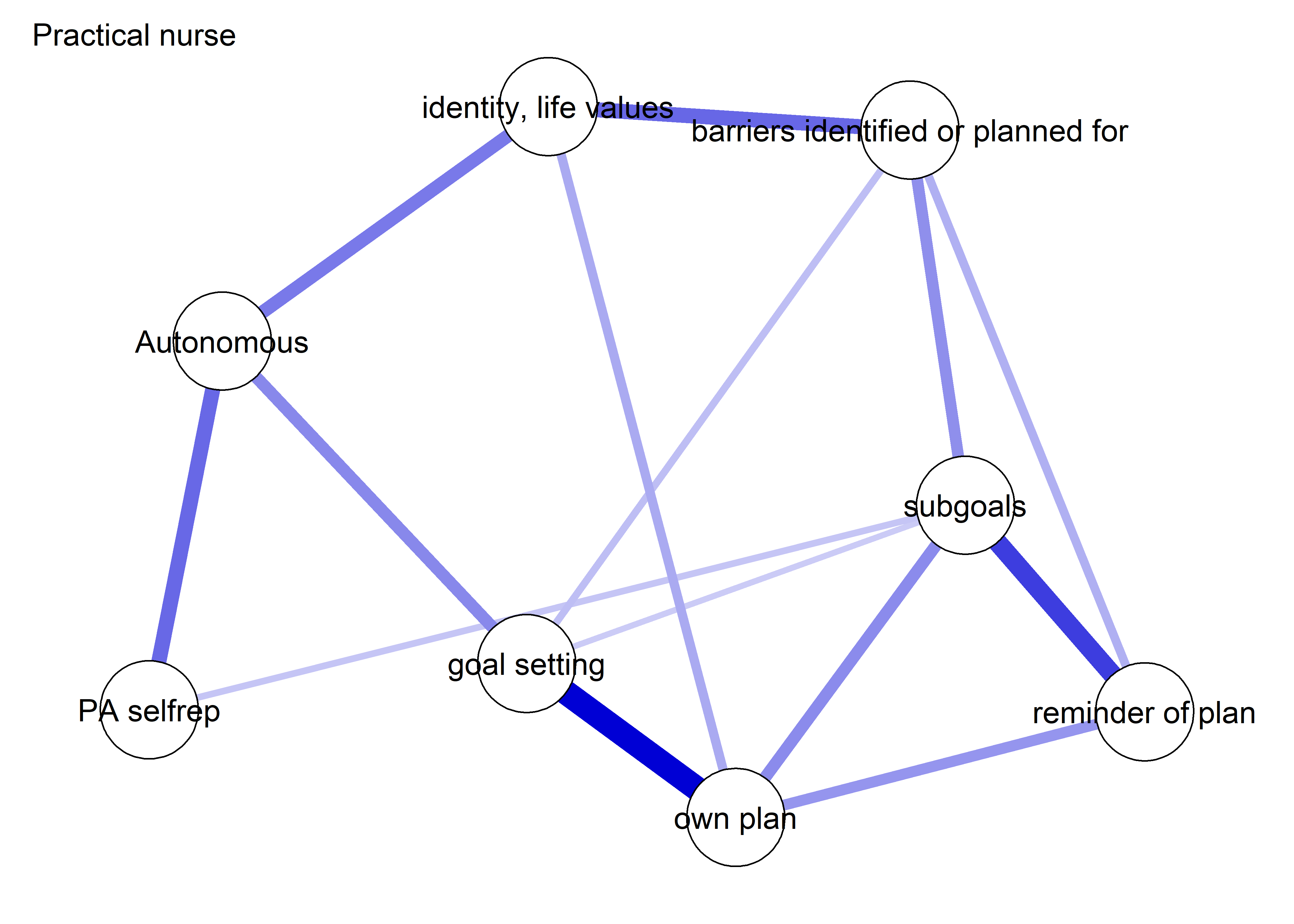
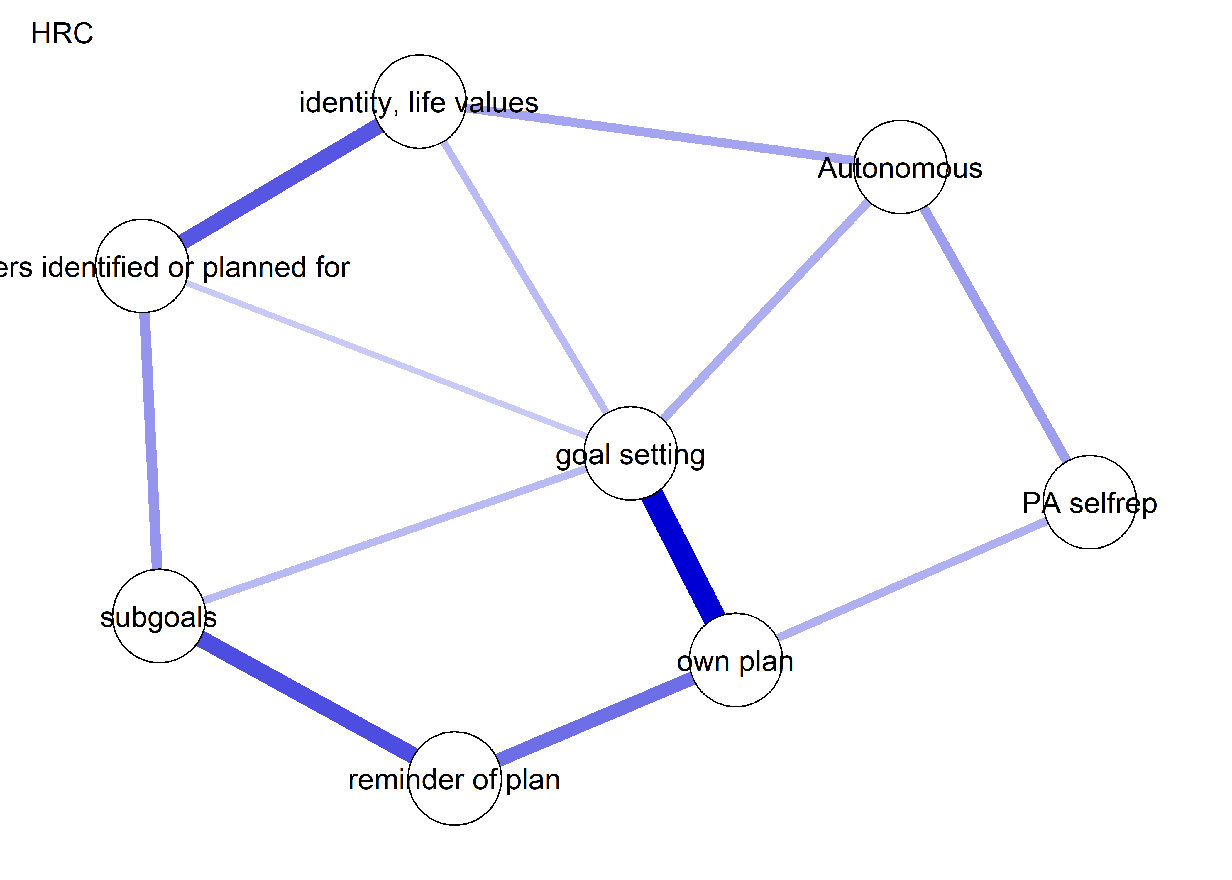
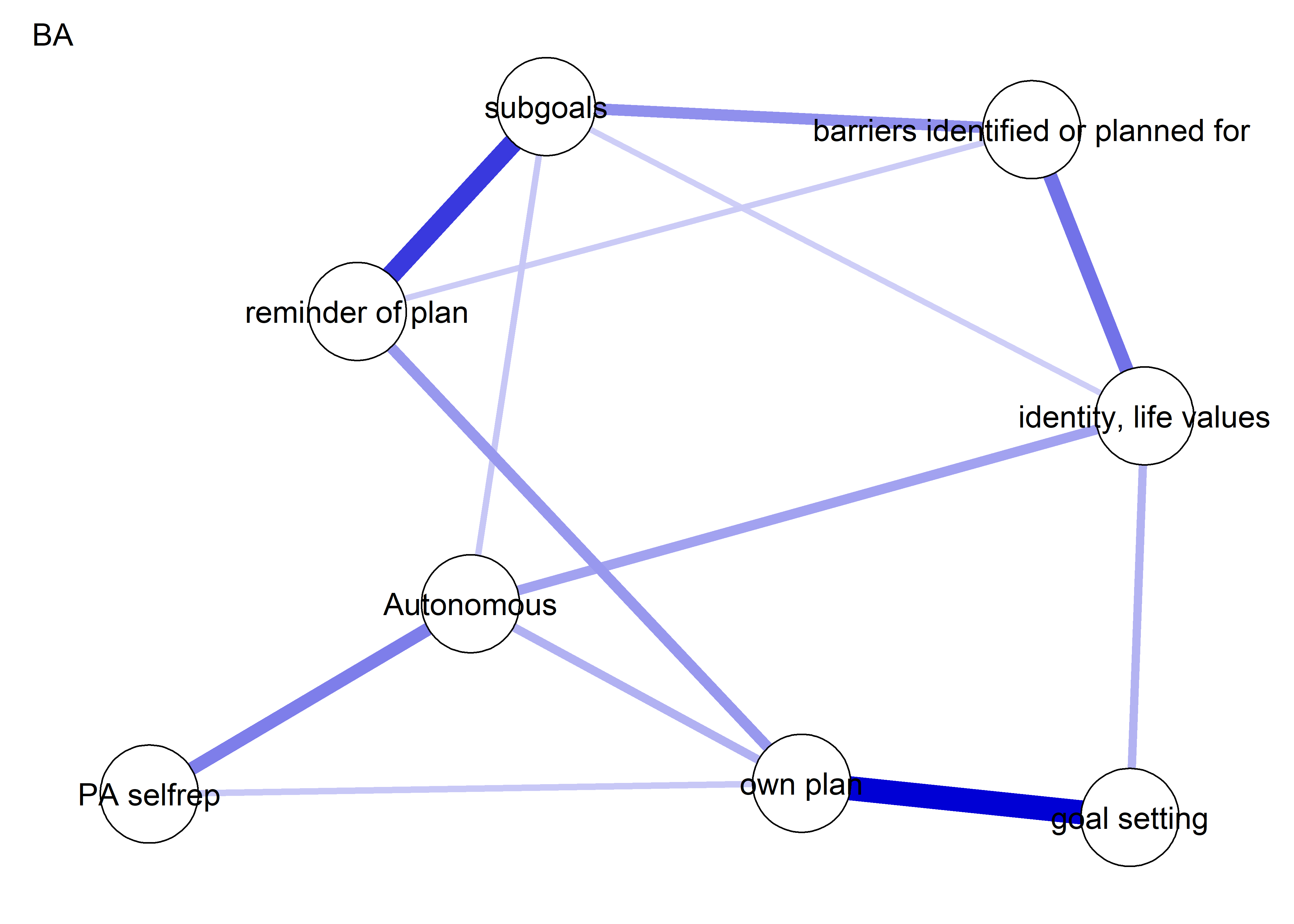
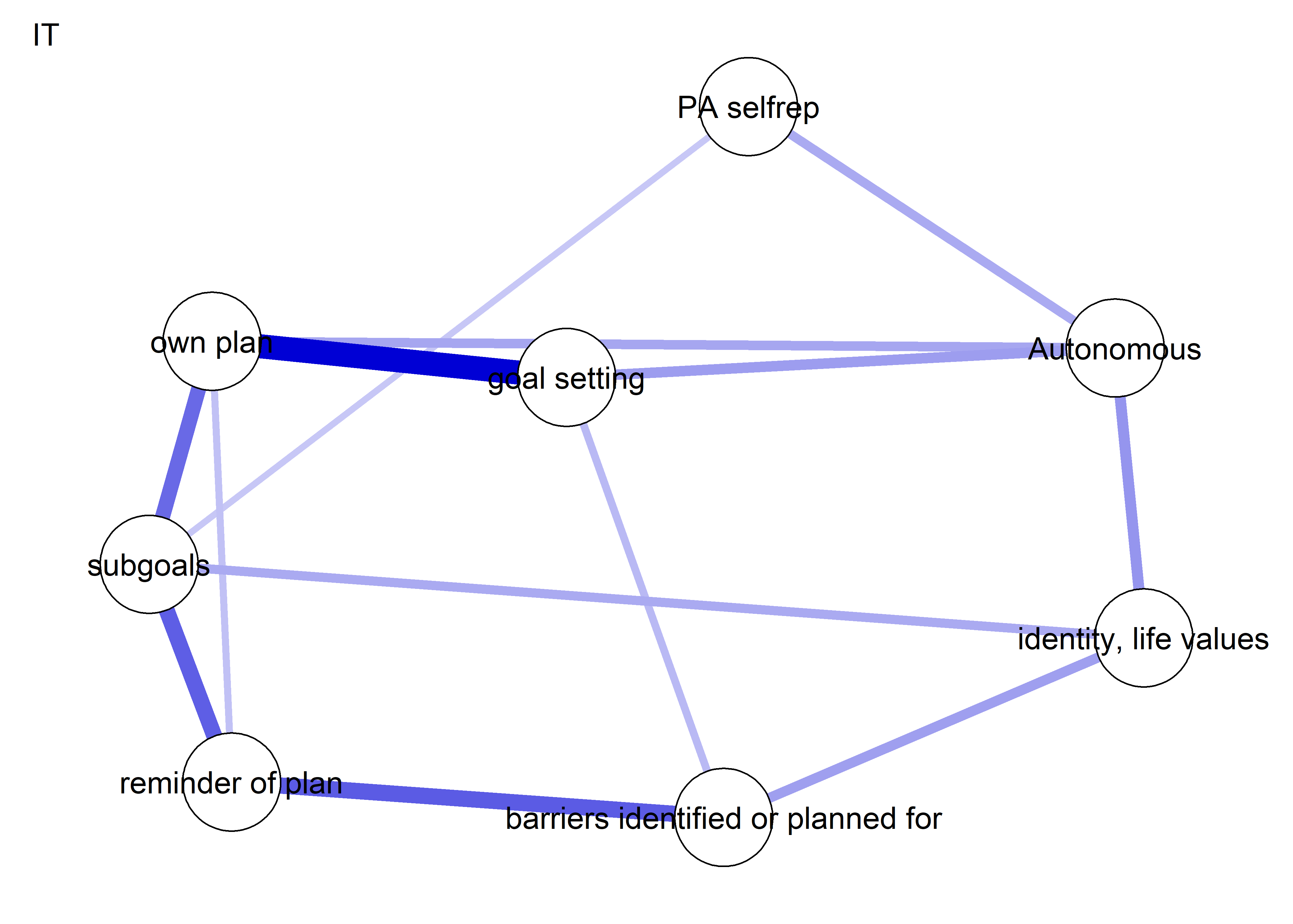
maxedge <- max(c(graph_Nur$graphAttributes$Graph$maximum,
                 graph_HRC$graphAttributes$Graph$maximum,
                 graph_BA$graphAttributes$Graph$maximum,
                 graph_IT$graphAttributes$Graph$maximum))

L <- qgraph::averageLayout(graph_Nur, graph_HRC, graph_BA, graph_IT)

layout(matrix(1:4, nrow = 2, byrow = TRUE))
graph_Nur <- plot(network_Nur, layout=L, cut=0, label.scale = FALSE, title = "Practical nurse",
                  maximum = maxedge)
graph_HRC <- plot(network_HRC, layout=L, cut=0, label.scale = FALSE, title = "HRC",
                  maximum = maxedge)
graph_BA <- plot(network_BA, layout=L, cut=0, label.scale = FALSE, title = "BA",
                 maximum = maxedge)
graph_IT <- plot(network_IT, layout=L, cut=0, label.scale = FALSE, title = "IT",
                 maximum = maxedge)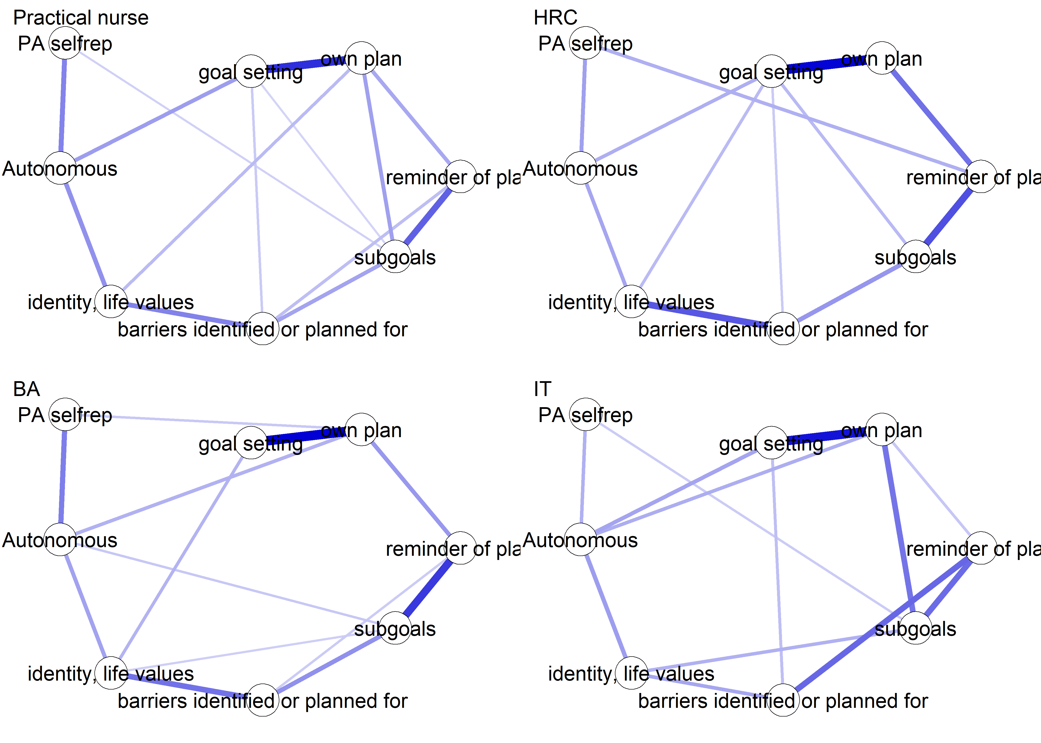
# nct_results <- NetworkComparisonTest::NCT(heterogeneity_Nur, heterogeneity_IT, it=1000, binary.data=FALSE, paired=FALSE, test.edges=TRUE,
# edges='all', progressbar=TRUE)
#
# save(nct_results, file = "./Rdata_files/nct_results.Rdata")
load("./Rdata_files/nct_results.Rdata")
print("These are the sizes of educational tracks:")
## [1] "These are the sizes of educational tracks:"
combinedAgreementBcts_tracks_df %>% dplyr::group_by(track) %>% summarise(n = n()) %>%
papaja::apa_table()
## <caption>(\#tab:combinedAgreementBcts-heterogeneity-nct)</caption>
##
## <caption>**</caption>
##
##
##
## track n
## ------ ----
## Other 24
## IT 171
## BA 276
## HRC 211
## Nur 402
## NA 82
print("Similarity")
## [1] "Similarity"
cat("Correlation between Nur and IT edge strengths:", cor(qgraph::centrality(network_Nur)$InDegree, qgraph::centrality(network_IT)$InDegree))
## Correlation between Nur and IT edge strengths: 0.9558435
cat("Correlation between Nur and IT networks:", cor(network_Nur$graph[lower.tri(network_Nur$graph)], network_IT$graph[lower.tri(network_Nur$graph)], method="spearman"))
## Correlation between Nur and IT networks: 0.7463299
print("Difference")
## [1] "Difference"
cat("P-value for the test of identical network structure:", nct_results$nwinv.pval)
## P-value for the test of identical network structure: 0.35
cat("P-value for the test of identical connectivity in networks:", nct_results$glstrinv.pval)
## P-value for the test of identical connectivity in networks: 0.018
nct_results$einv.pvals %>%
papaja::apa_table(caption = "p-values on difference test in edges between Nur and IT")
## <caption>(\#tab:combinedAgreementBcts-heterogeneity-nct)</caption>
##
## <caption>*p-values on difference test in edges between Nur and IT*</caption>
##
##
##
## Var1 Var2 p-value
## ---- ------------------------------ ------------------------------ --------
## 20 goal setting own plan 1.00
## 39 goal setting plan by other 1.00
## 40 own plan plan by other 1.00
## 58 goal setting reminder of plan 1.00
## 59 own plan reminder of plan 1.00
## 60 plan by other reminder of plan 1.00
## 77 goal setting subgoals 1.00
## 78 own plan subgoals 1.00
## 79 plan by other subgoals 1.00
## 80 reminder of plan subgoals 1.00
## 96 goal setting trying new PA 1.00
## 97 own plan trying new PA 1.00
## 98 plan by other trying new PA 1.00
## 99 reminder of plan trying new PA 1.00
## 100 subgoals trying new PA 1.00
## 115 goal setting barrier identification 1.00
## 116 own plan barrier identification 1.00
## 117 plan by other barrier identification 1.00
## 118 reminder of plan barrier identification 1.00
## 119 subgoals barrier identification 1.00
## 120 trying new PA barrier identification 1.00
## 134 goal setting problem solving 1.00
## 135 own plan problem solving 1.00
## 136 plan by other problem solving 1.00
## 137 reminder of plan problem solving 1.00
## 138 subgoals problem solving 1.00
## 139 trying new PA problem solving 1.00
## 140 barrier identification problem solving 1.00
## 153 goal setting PA identity reflection 1.00
## 154 own plan PA identity reflection 1.00
## 155 plan by other PA identity reflection 1.00
## 156 reminder of plan PA identity reflection 1.00
## 157 subgoals PA identity reflection 1.00
## 158 trying new PA PA identity reflection 1.00
## 159 barrier identification PA identity reflection 1.00
## 160 problem solving PA identity reflection 1.00
## 172 goal setting aligning PA with life values 1.00
## 173 own plan aligning PA with life values 1.00
## 174 plan by other aligning PA with life values 1.00
## 175 reminder of plan aligning PA with life values 1.00
## 176 subgoals aligning PA with life values 1.00
## 177 trying new PA aligning PA with life values 1.00
## 178 barrier identification aligning PA with life values 0.84
## 179 problem solving aligning PA with life values 1.00
## 180 PA identity reflection aligning PA with life values 1.00
## 191 goal setting remind of PA benefits 1.00
## 192 own plan remind of PA benefits 1.00
## 193 plan by other remind of PA benefits 1.00
## 194 reminder of plan remind of PA benefits 1.00
## 195 subgoals remind of PA benefits 1.00
## 196 trying new PA remind of PA benefits 1.00
## 197 barrier identification remind of PA benefits 1.00
## 198 problem solving remind of PA benefits 1.00
## 199 PA identity reflection remind of PA benefits 1.00
## 200 aligning PA with life values remind of PA benefits 1.00
## 210 goal setting self-monitor (paper) 1.00
## 211 own plan self-monitor (paper) 1.00
## 212 plan by other self-monitor (paper) 1.00
## 213 reminder of plan self-monitor (paper) 1.00
## 214 subgoals self-monitor (paper) 1.00
## 215 trying new PA self-monitor (paper) 1.00
## 216 barrier identification self-monitor (paper) 1.00
## 217 problem solving self-monitor (paper) 1.00
## 218 PA identity reflection self-monitor (paper) 1.00
## 219 aligning PA with life values self-monitor (paper) 1.00
## 220 remind of PA benefits self-monitor (paper) 1.00
## 229 goal setting self-monitor (app) 1.00
## 230 own plan self-monitor (app) 1.00
## 231 plan by other self-monitor (app) 0.17
## 232 reminder of plan self-monitor (app) 1.00
## 233 subgoals self-monitor (app) 1.00
## 234 trying new PA self-monitor (app) 1.00
## 235 barrier identification self-monitor (app) 1.00
## 236 problem solving self-monitor (app) 1.00
## 237 PA identity reflection self-monitor (app) 1.00
## 238 aligning PA with life values self-monitor (app) 1.00
## 239 remind of PA benefits self-monitor (app) 1.00
## 240 self-monitor (paper) self-monitor (app) 1.00
## 248 goal setting memory cues 1.00
## 249 own plan memory cues 1.00
## 250 plan by other memory cues 1.00
## 251 reminder of plan memory cues 1.00
## 252 subgoals memory cues 1.00
## 253 trying new PA memory cues 1.00
## 254 barrier identification memory cues 1.00
## 255 problem solving memory cues 1.00
## 256 PA identity reflection memory cues 1.00
## 257 aligning PA with life values memory cues 1.00
## 258 remind of PA benefits memory cues 1.00
## 259 self-monitor (paper) memory cues 1.00
## 260 self-monitor (app) memory cues 1.00
## 267 goal setting goal review 0.84
## 268 own plan goal review 1.00
## 269 plan by other goal review 1.00
## 270 reminder of plan goal review 1.00
## 271 subgoals goal review 1.00
## 272 trying new PA goal review 1.00
## 273 barrier identification goal review 1.00
## 274 problem solving goal review 1.00
## 275 PA identity reflection goal review 1.00
## 276 aligning PA with life values goal review 1.00
## 277 remind of PA benefits goal review 1.00
## 278 self-monitor (paper) goal review 0.17
## 279 self-monitor (app) goal review 1.00
## 280 memory cues goal review 1.00
## 286 goal setting personal relevance reflection 1.00
## 287 own plan personal relevance reflection 1.00
## 288 plan by other personal relevance reflection 1.00
## 289 reminder of plan personal relevance reflection 1.00
## 290 subgoals personal relevance reflection 1.00
## 291 trying new PA personal relevance reflection 1.00
## 292 barrier identification personal relevance reflection 1.00
## 293 problem solving personal relevance reflection 1.00
## 294 PA identity reflection personal relevance reflection 1.00
## 295 aligning PA with life values personal relevance reflection 1.00
## 296 remind of PA benefits personal relevance reflection 1.00
## 297 self-monitor (paper) personal relevance reflection 1.00
## 298 self-monitor (app) personal relevance reflection 1.00
## 299 memory cues personal relevance reflection 1.00
## 300 goal review personal relevance reflection 1.00
## 305 goal setting environmental changes (home) 1.00
## 306 own plan environmental changes (home) 1.00
## 307 plan by other environmental changes (home) 1.00
## 308 reminder of plan environmental changes (home) 1.00
## 309 subgoals environmental changes (home) 1.00
## 310 trying new PA environmental changes (home) 1.00
## 311 barrier identification environmental changes (home) 1.00
## 312 problem solving environmental changes (home) 1.00
## 313 PA identity reflection environmental changes (home) 1.00
## 314 aligning PA with life values environmental changes (home) 1.00
## 315 remind of PA benefits environmental changes (home) 1.00
## 316 self-monitor (paper) environmental changes (home) 1.00
## 317 self-monitor (app) environmental changes (home) 1.00
## 318 memory cues environmental changes (home) 1.00
## 319 goal review environmental changes (home) 1.00
## 320 personal relevance reflection environmental changes (home) 1.00
## 324 goal setting social support 1.00
## 325 own plan social support 1.00
## 326 plan by other social support 1.00
## 327 reminder of plan social support 1.00
## 328 subgoals social support 1.00
## 329 trying new PA social support 1.00
## 330 barrier identification social support 1.00
## 331 problem solving social support 1.00
## 332 PA identity reflection social support 1.00
## 333 aligning PA with life values social support 1.00
## 334 remind of PA benefits social support 1.00
## 335 self-monitor (paper) social support 1.00
## 336 self-monitor (app) social support 1.00
## 337 memory cues social support 1.00
## 338 goal review social support 1.00
## 339 personal relevance reflection social support 1.00
## 340 environmental changes (home) social support 1.00
## 343 goal setting failure contemplated 1.00
## 344 own plan failure contemplated 1.00
## 345 plan by other failure contemplated 1.00
## 346 reminder of plan failure contemplated 1.00
## 347 subgoals failure contemplated 1.00
## 348 trying new PA failure contemplated 1.00
## 349 barrier identification failure contemplated 1.00
## 350 problem solving failure contemplated 1.00
## 351 PA identity reflection failure contemplated 1.00
## 352 aligning PA with life values failure contemplated 1.00
## 353 remind of PA benefits failure contemplated 1.00
## 354 self-monitor (paper) failure contemplated 1.00
## 355 self-monitor (app) failure contemplated 1.00
## 356 memory cues failure contemplated 1.00
## 357 goal review failure contemplated 1.00
## 358 personal relevance reflection failure contemplated 1.00
## 359 environmental changes (home) failure contemplated 0.00
## 360 social support failure contemplated 1.00
cat("Number of edges, which appear different (p<0.05):", sum(nct_results$einv.pvals$"p-value" < 0.05))
## Number of edges, which appear different (p<0.05): 1Ising networks
Plot with only the BCTs
Prepare and dichotomise data (lots of skew in distributions).
nItems <- 19

bctdf <- df %>% dplyr::select(id,
  intervention,
  group,
  school,
  girl,
  'goal setting' = PA_agreementDependentBCT_01_T1,
  'own plan' = PA_agreementDependentBCT_02_T1,
  'plan by other' = PA_agreementDependentBCT_03_T1,
  'reminder of plan' = PA_agreementDependentBCT_04_T1,
  'subgoals' = PA_agreementDependentBCT_05_T1,
  'trying new PA' = PA_agreementDependentBCT_06_T1,
  'barrier identification' = PA_agreementDependentBCT_07_T1,
  'problem solving' = PA_agreementDependentBCT_08_T1,
  'PA identity reflection' = PA_agreementDependentBCT_09_T1,
  'aligning PA with life values' = PA_agreementDependentBCT_10_T1,
  'remind of PA benefits' = PA_frequencyDependentBCT_01_T1,
  'self-monitor (paper)' = PA_frequencyDependentBCT_02_T1,
  'self-monitor (app)' = PA_frequencyDependentBCT_03_T1,
  'memory cues' = PA_frequencyDependentBCT_04_T1,
  'goal review' = PA_frequencyDependentBCT_05_T1,
  'personal relevance reflection' = PA_frequencyDependentBCT_06_T1,
  'environmental changes (home)' = PA_frequencyDependentBCT_07_T1,
  'social support' = PA_frequencyDependentBCT_08_T1,
  'failure contemplated' = PA_frequencyDependentBCT_09_T1) %>%
 mutate(
  'goal setting' = ifelse(`goal setting` == 1, 0, 1),
  'own plan' = ifelse(`own plan` == 1, 0, 1),
  'plan by other' = ifelse(`plan by other` == 1, 0, 1),
  'reminder of plan' = ifelse(`reminder of plan` == 1, 0, 1),
  'subgoals' = ifelse(`subgoals` == 1, 0, 1),
  'trying new PA' = ifelse(`trying new PA` == 1, 0, 1),
  'barrier identification' = ifelse(`barrier identification` == 1, 0, 1),
  'problem solving' = ifelse(`problem solving` == 1, 0, 1),
  'PA identity reflection' = ifelse(`PA identity reflection` == 1, 0, 1),
  'aligning PA with life values' = ifelse(`aligning PA with life values` == 1, 0, 1),
  'remind of PA benefits' = ifelse(`remind of PA benefits` == 1, 0, 1),
  'self-monitor (paper)' = ifelse(`self-monitor (paper)` == 1, 0, 1),
  'self-monitor (app)' = ifelse(`self-monitor (app)` == 1, 0, 1),
  'memory cues' = ifelse(`memory cues` == 1, 0, 1),
  'goal review' = ifelse(`goal review` == 1, 0, 1),
  'personal relevance reflection' = ifelse(`personal relevance reflection` == 1, 0, 1),
  'environmental changes (home)' = ifelse(`environmental changes (home)` == 1, 0, 1),
  'social support' = ifelse(`social support` == 1, 0, 1),
  'failure contemplated' = ifelse(`failure contemplated` == 1, 0, 1))

S.boys <- bctdf %>% filter(girl == "boy") %>% dplyr::select(`goal setting`:ncol(bctdf)) %>% na.omit(.)
S.girls <- bctdf %>% filter(girl == "girl") %>% dplyr::select(`goal setting`:ncol(bctdf)) %>% na.omit(.)
nwBoys <- bootnet::estimateNetwork(S.boys, default="IsingFit")
##
  |
  |                                                                 |   0%
  |
  |===                                                              |   5%
  |
  |=======                                                          |  11%
  |
  |==========                                                       |  16%
  |
  |==============                                                   |  21%
  |
  |=================                                                |  26%
  |
  |=====================                                            |  32%
  |
  |========================                                         |  37%
  |
  |===========================                                      |  42%
  |
  |===============================                                  |  47%
  |
  |==================================                               |  53%
  |
  |======================================                           |  58%
  |
  |=========================================                        |  63%
  |
  |============================================                     |  68%
  |
  |================================================                 |  74%
  |
  |===================================================              |  79%
  |
  |=======================================================          |  84%
  |
  |==========================================================       |  89%
  |
  |==============================================================   |  95%
  |
  |=================================================================| 100%
nwGirls <- bootnet::estimateNetwork(S.girls, default="IsingFit")
##
  |
  |                                                                 |   0%
  |
  |===                                                              |   5%
  |
  |=======                                                          |  11%
  |
  |==========                                                       |  16%
  |
  |==============                                                   |  21%
  |
  |=================                                                |  26%
  |
  |=====================                                            |  32%
  |
  |========================                                         |  37%
  |
  |===========================                                      |  42%
  |
  |===============================                                  |  47%
  |
  |==================================                               |  53%
  |
  |======================================                           |  58%
  |
  |=========================================                        |  63%
  |
  |============================================                     |  68%
  |
  |================================================                 |  74%
  |
  |===================================================              |  79%
  |
  |=======================================================          |  84%
  |
  |==========================================================       |  89%
  |
  |==============================================================   |  95%
  |
  |=================================================================| 100%

# Create means for filling nodes

girlmeans <- bctdf %>%
  dplyr::filter(girl == "girl") %>%
  summarise_at(vars(-(id:girl)),
  funs(mean(., na.rm = TRUE)))

boymeans <- bctdf %>%
  dplyr::filter(girl == "boy") %>%
  summarise_at(vars(-(id:girl)),
  funs(mean(., na.rm = TRUE)))
For girls and boys.
# Find average layout for comparability and plot graphs next to each other

Layout <- qgraph::averageLayout(nwGirls, nwBoys)

layout(t(1:2))

plot(nwGirls, layout = Layout, label.scale = FALSE, title = "Girls", label.cex = 0.75,
     pie = girlmeans,
     color = "skyblue",
     pieBorder = 1)

plot(nwBoys, layout = Layout, label.scale = FALSE, title = "Boys", label.cex = 0.75,
     pie = boymeans,
     color = "skyblue",
     pieBorder = 1)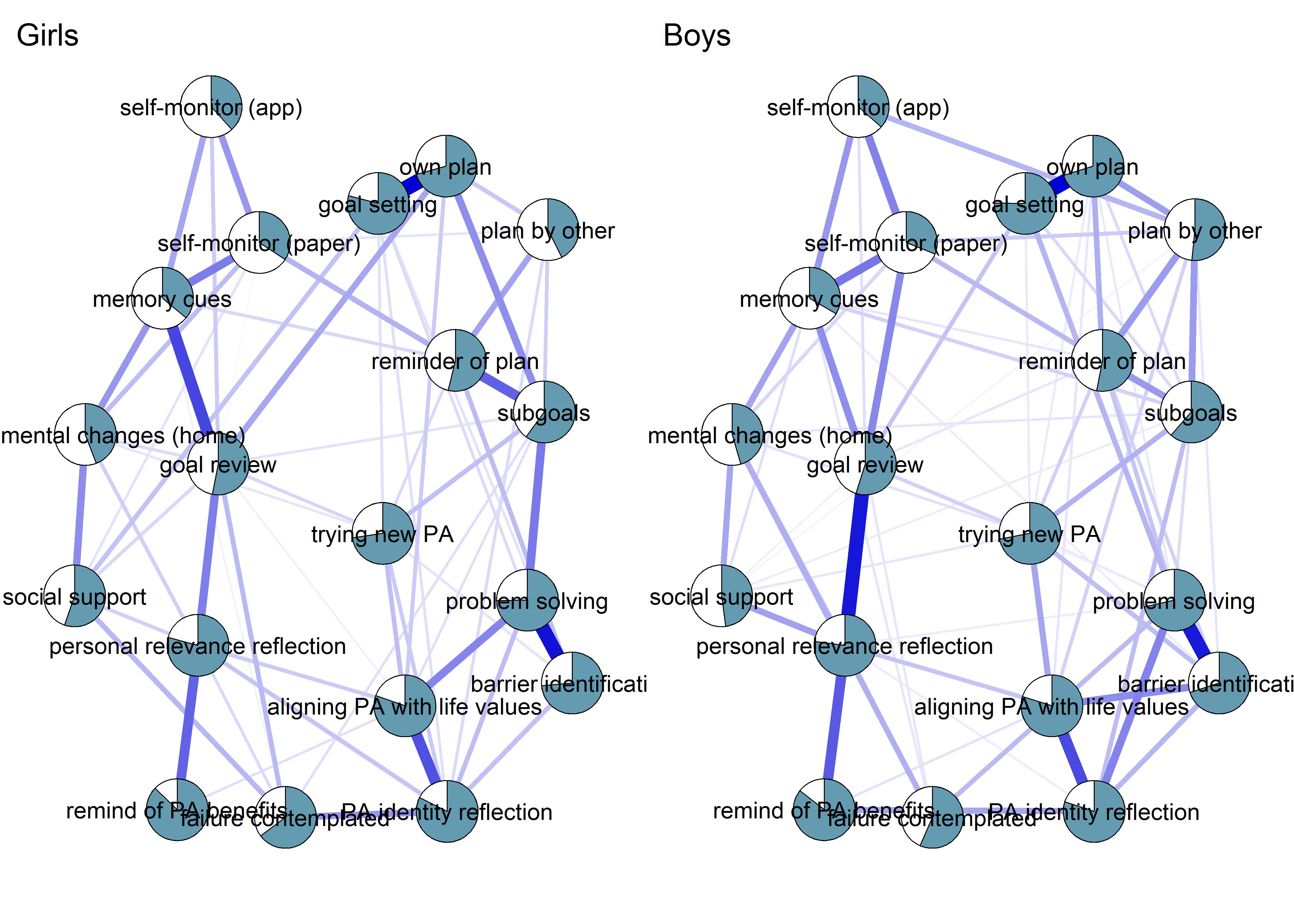
Network comparison test: boys vs. girls
# nct_results2 <- NetworkComparisonTest::NCT(S.boys, S.girls, it=1000, binary.data=TRUE, paired=FALSE, test.edges=TRUE, edges='all', progressbar=TRUE)
#
# save(nct_results2, file = "./Rdata_files/nct_results2.Rdata")
load("./Rdata_files/nct_results2.Rdata")

cat("P-value of network structure difference test:", nct_results2$nwinv.pval)
P-value of network structure difference test: 0.361
P-value of global connectivity difference test: 0.02
nct_results2$einv.pvals %>%
  dplyr::filter(`p-value` < 1) %>%      #p values testing diffs for all individual edges
knitr::kable(caption = "P-values for edge strength differences among boys and girls. Omitted edges where p = 1.")| Var1 | Var2 | p-value |
|---|---|---|
| plan by other | self-monitor (app) | 0.340 |
| goal setting | goal review | 0.840 |
| self-monitor (paper) | goal review | 0.676 |
| environmental changes (home) | failure contemplated | 0.000 |
For all participants.
S.total <- bctdf %>% dplyr::select(6:ncol(bctdf))
nwBCT <- bootnet::estimateNetwork(S.total, default="IsingFit")
##
  |
  |                                                                 |   0%
  |
  |===                                                              |   5%
  |
  |=======                                                          |  11%
  |
  |==========                                                       |  16%
  |
  |==============                                                   |  21%
  |
  |=================                                                |  26%
  |
  |=====================                                            |  32%
  |
  |========================                                         |  37%
  |
  |===========================                                      |  42%
  |
  |===============================                                  |  47%
  |
  |==================================                               |  53%
  |
  |======================================                           |  58%
  |
  |=========================================                        |  63%
  |
  |============================================                     |  68%
  |
  |================================================                 |  74%
  |
  |===================================================              |  79%
  |
  |=======================================================          |  84%
  |
  |==========================================================       |  89%
  |
  |==============================================================   |  95%
  |
  |=================================================================| 100%

# Create means for filling nodes
piefill <- S.total %>%
  summarise_all(funs(mean(., na.rm = TRUE)))

# Plot network
Ising_fit <- plot(nwBCT, layout = "spring",
     label.scale = FALSE, title = "Ising fit", label.cex = 0.75,
     pie = piefill,
     color = "skyblue",
     pieBorder = 1,
     # DoNotPlot = TRUE
     )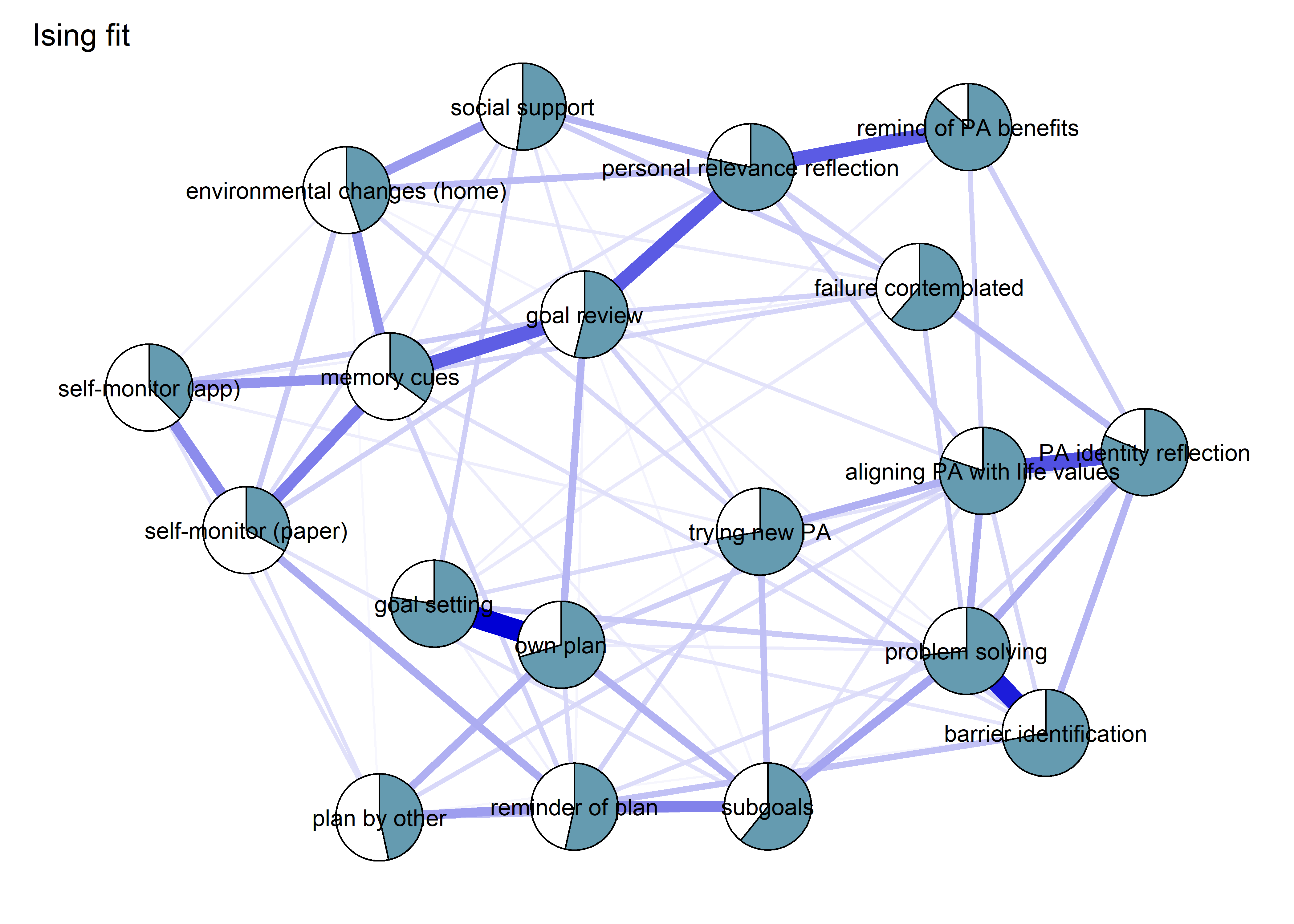
# # Estimate ising network without regularisation DOES NOT CONVERGE --> OMITTED
# nwBCT_nonreg <- bootnet::estimateNetwork(S.total, default="IsingSampler")
#
# nonreg <- plot(nwBCT_nonreg, layout = "spring",
#      label.scale = FALSE, title = "Non-regularised Ising model", label.cex = 0.75,
#      pie = piefill,
#      color = "skyblue",
#      pieBorder = 1,
#      DoNotPlot = TRUE)
#
# layout_allParticipants <- qgraph::averageLayout(Ising_fit, nonreg)
#
# # Plot network
# plot(nwBCT, layout = "layout_allParticipants",
#      label.scale = FALSE, title = "Ising fit", label.cex = 0.75,
#      pie = piefill,
#      color = "skyblue",
#      pieBorder = 1)
#
# plot(nwBCT_nonreg, layout = "layout_allParticipants",
#      label.scale = FALSE, title = "Non-regularised Ising model", label.cex = 0.75,
#      pie = piefill,
#      color = "skyblue",
#      pieBorder = 1)
Ising network Combined items
nItems <- 17

bctdf <- df %>% dplyr::select(id,
  intervention,
  group,
  school,
  girl,
  'goal setting' = PA_agreementDependentBCT_01_T1,
  'own plan' = PA_agreementDependentBCT_02_T1,
  'plan by other' = PA_agreementDependentBCT_03_T1,
  'reminder of plan' = PA_agreementDependentBCT_04_T1,
  'subgoals' = PA_agreementDependentBCT_05_T1,
  'trying new PA' = PA_agreementDependentBCT_06_T1,
  'barrier identification' = PA_agreementDependentBCT_07_T1,
  'problem solving' = PA_agreementDependentBCT_08_T1,
  'PA identity reflection' = PA_agreementDependentBCT_09_T1,
  'aligning PA with life values' = PA_agreementDependentBCT_10_T1,
  'remind of PA benefits' = PA_frequencyDependentBCT_01_T1,
  'self-monitor (paper)' = PA_frequencyDependentBCT_02_T1,
  'self-monitor (app)' = PA_frequencyDependentBCT_03_T1,
#  'memory cues' = PA_frequencyDependentBCT_04_T1,
  'goal review' = PA_frequencyDependentBCT_05_T1,
  'personal relevance reflection' = PA_frequencyDependentBCT_06_T1,
  'environmental changes (home)' = PA_frequencyDependentBCT_07_T1,
  'social support' = PA_frequencyDependentBCT_08_T1,
  'failure contemplated' = PA_frequencyDependentBCT_09_T1) %>%
 mutate(
  'goal setting' = ifelse(`goal setting` == 1, 0, 1),
  'own plan' = ifelse(`own plan` == 1 & `plan by other` == 1, 0, 1),
  'reminder of plan' = ifelse(`reminder of plan` == 1, 0, 1),
  'subgoals' = ifelse(`subgoals` == 1, 0, 1),
  'trying new PA' = ifelse(`trying new PA` == 1, 0, 1),
  'barrier identification' = ifelse(`barrier identification` == 1, 0, 1),
  'problem solving' = ifelse(`problem solving` == 1, 0, 1),
  'PA identity reflection' = ifelse(`PA identity reflection` == 1, 0, 1),
  'aligning PA with life values' = ifelse(`aligning PA with life values` == 1, 0, 1),
  'remind of PA benefits' = ifelse(`remind of PA benefits` == 1, 0, 1),
  'self-monitor' = ifelse(`self-monitor (paper)` == 1 & `self-monitor (app)` == 1, 0, 1),
#  'memory cues' = ifelse(`memory cues` == 1, 0, 1),
  'goal review' = ifelse(`goal review` == 1, 0, 1),
  'personal relevance reflection' = ifelse(`personal relevance reflection` == 1, 0, 1),
  'environmental changes (home)' = ifelse(`environmental changes (home)` == 1, 0, 1),
  'social support' = ifelse(`social support` == 1, 0, 1),
  'failure contemplated' = ifelse(`failure contemplated` == 1, 0, 1)) %>%
  dplyr::select(-`self-monitor (paper)`, -`self-monitor (app)`, -`plan by other`) %>%
  mutate_all(as.numeric)

# Network for all participants

S.total <- bctdf %>% dplyr::select(6:ncol(bctdf))
nwBCT <- bootnet::estimateNetwork(S.total, default="IsingFit")
##
  |
  |                                                                 |   0%
  |
  |====                                                             |   6%
  |
  |========                                                         |  12%
  |
  |============                                                     |  19%
  |
  |================                                                 |  25%
  |
  |====================                                             |  31%
  |
  |========================                                         |  38%
  |
  |============================                                     |  44%
  |
  |================================                                 |  50%
  |
  |=====================================                            |  56%
  |
  |=========================================                        |  62%
  |
  |=============================================                    |  69%
  |
  |=================================================                |  75%
  |
  |=====================================================            |  81%
  |
  |=========================================================        |  88%
  |
  |=============================================================    |  94%
  |
  |=================================================================| 100%

# Create means for filling nodes
piefill <- S.total %>%
  summarise_all(funs(mean(., na.rm = TRUE)))

# Plot network
plot(nwBCT, layout = "spring", label.scale = FALSE, title = "Ising fit", label.cex = 0.75,
     pie = piefill,
     color = "skyblue",
     pieBorder = 1)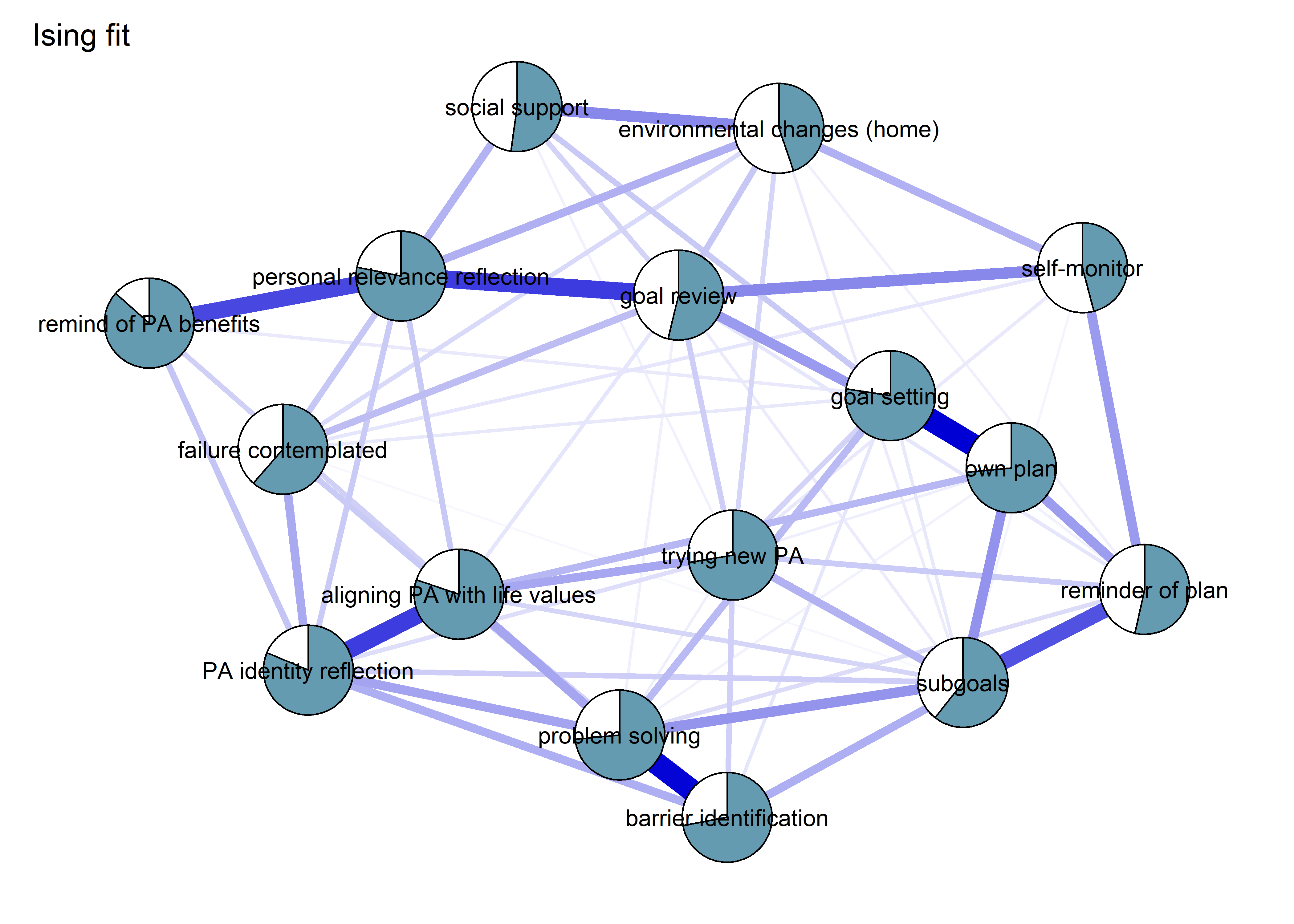
# # Estimate ising network without regularisation
# nwBCT_nonreg <- bootnet::estimateNetwork(S.total, default="IsingSampler")
#
# plot(nwBCT_nonreg, layout = "spring", label.scale = FALSE, title = "Non-regularised Ising model", label.cex = 0.75,
#      pie = piefill,
#      color = "skyblue",
#      pieBorder = 1)
Centrality and stability
onlyCombinedBctsIsing <- nwBCT_ggm

onlyCombinedBctsIsing_centralityPlot <- qgraph::centralityPlot(onlyCombinedBctsIsing)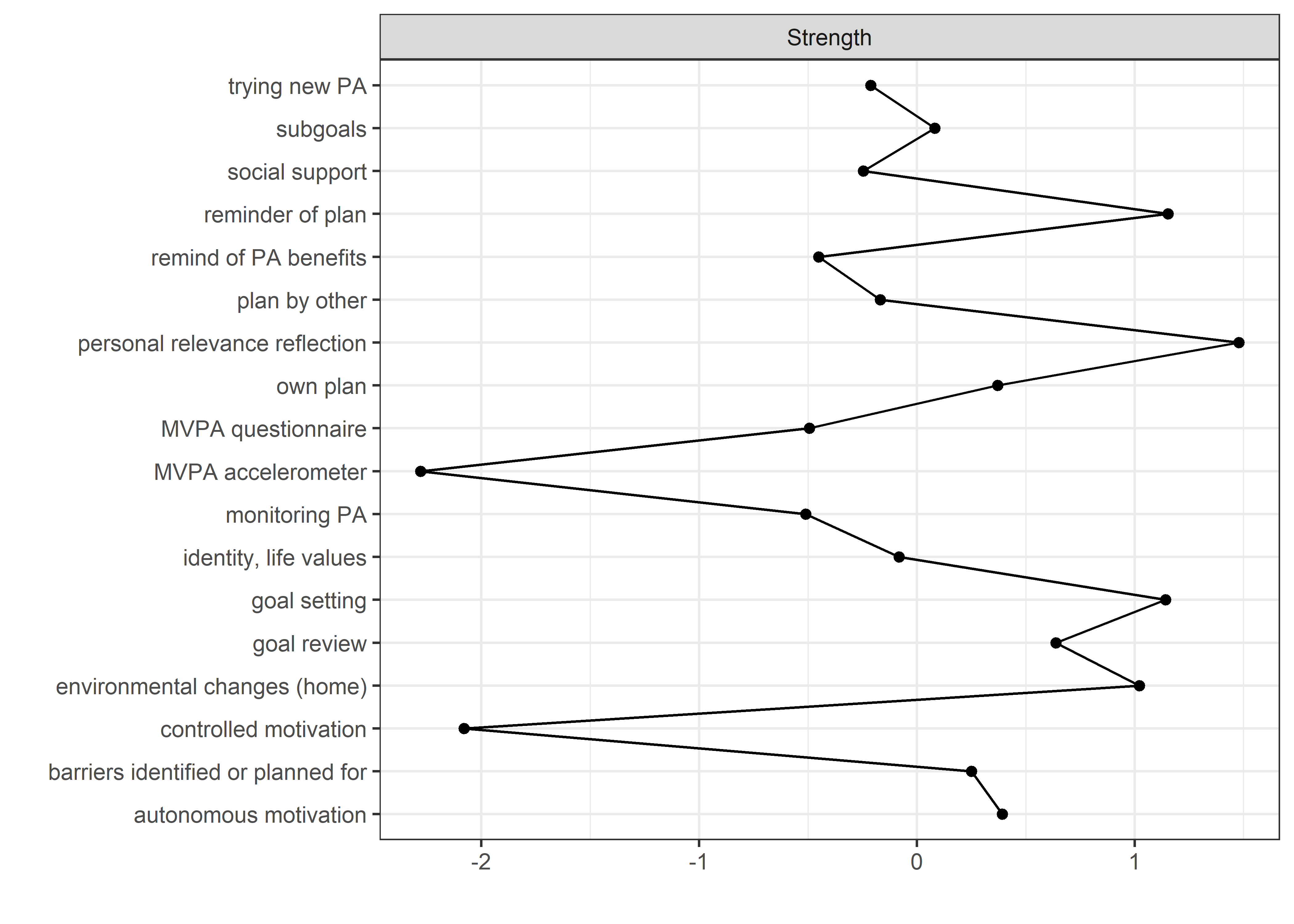
qgraph::centrality(onlyCombinedBctsIsing)$InDegree
##                 MVPA questionnaire                 MVPA accelerometer
##                          0.8556311                          0.2966012
##              autonomous motivation              controlled motivation
##                          1.1333014                          0.3589353
##                       goal setting                           own plan
##                          1.3678574                          1.1263288
##                      plan by other                   reminder of plan
##                          0.9578744                          1.3714270
##                           subgoals                      trying new PA
##                          1.0362904                          0.9438976
##              remind of PA benefits                        goal review
##                          0.8689656                          1.2104140
##      personal relevance reflection       environmental changes (home)
##                          1.4734305                          1.3303871
##                     social support barriers identified or planned for
##                          0.9332922                          1.0887339
##              identity, life values                      monitoring PA
##                          0.9847564                          0.8505746
scale(qgraph::centrality(onlyCombinedBctsIsing)$InDegree)
##                                           [,1]
## MVPA questionnaire                 -0.49444010
## MVPA accelerometer                 -2.27941234
## autonomous motivation               0.39215589
## controlled motivation              -2.08038073
## goal setting                        1.14108898
## own plan                            0.36989258
## plan by other                      -0.16797929
## reminder of plan                    1.15248686
## subgoals                            0.08240178
## trying new PA                      -0.21260670
## remind of PA benefits              -0.45186342
## goal review                         0.63837506
## personal relevance reflection       1.47818218
## environmental changes (home)        1.02144701
## social support                     -0.24646966
## barriers identified or planned for  0.24985280
## identity, life values              -0.08214548
## monitoring PA                      -0.51058543
## attr(,"scaled:center")
## [1] 1.010483
## attr(,"scaled:scale")
## [1] 0.3131869
qgraph::centrality(onlyCombinedBctsIsing)$Closeness
##                 MVPA questionnaire                 MVPA accelerometer
##                        0.005018704                        0.003676450
##              autonomous motivation              controlled motivation
##                        0.005824559                        0.003789143
##                       goal setting                           own plan
##                        0.005581152                        0.005569459
##                      plan by other                   reminder of plan
##                        0.005588982                        0.006540042
##                           subgoals                      trying new PA
##                        0.005680872                        0.005494895
##              remind of PA benefits                        goal review
##                        0.005592491                        0.006176219
##      personal relevance reflection       environmental changes (home)
##                        0.006312982                        0.005688125
##                     social support barriers identified or planned for
##                        0.005120706                        0.005263721
##              identity, life values                      monitoring PA
##                        0.005565475                        0.005826165
qgraph::centrality(onlyCombinedBctsIsing)$Betweenness
##                 MVPA questionnaire                 MVPA accelerometer
##                                 34                                  0
##              autonomous motivation              controlled motivation
##                                 24                                  2
##                       goal setting                           own plan
##                                 14                                 18
##                      plan by other                   reminder of plan
##                                 16                                 32
##                           subgoals                      trying new PA
##                                 10                                  4
##              remind of PA benefits                        goal review
##                                  6                                 10
##      personal relevance reflection       environmental changes (home)
##                                 34                                 34
##                     social support barriers identified or planned for
##                                 18                                 16
##              identity, life values                      monitoring PA
##                                  6                                 10

cor(qgraph::centrality(onlyCombinedBctsIsing)$InDegree, qgraph::centrality(onlyCombinedBctsIsing)$Betweenness,
    method = "spearman")
## [1] 0.5978302

# bootnet_stability_onlyCombinedBctsIsing <- bootnet::bootnet(onlyCombinedBctsIsing, stepwise = FALSE, nBoots=1000)
# save(bootnet_stability_onlyCombinedBctsIsing, file = "./Rdata_files/bootnet_stability_onlyCombinedBctsIsing.Rdata")
load("./Rdata_files/bootnet_stability_onlyCombinedBctsIsing.Rdata")

plot(bootnet_stability_onlyCombinedBctsIsing, labels = FALSE, order = "sample") 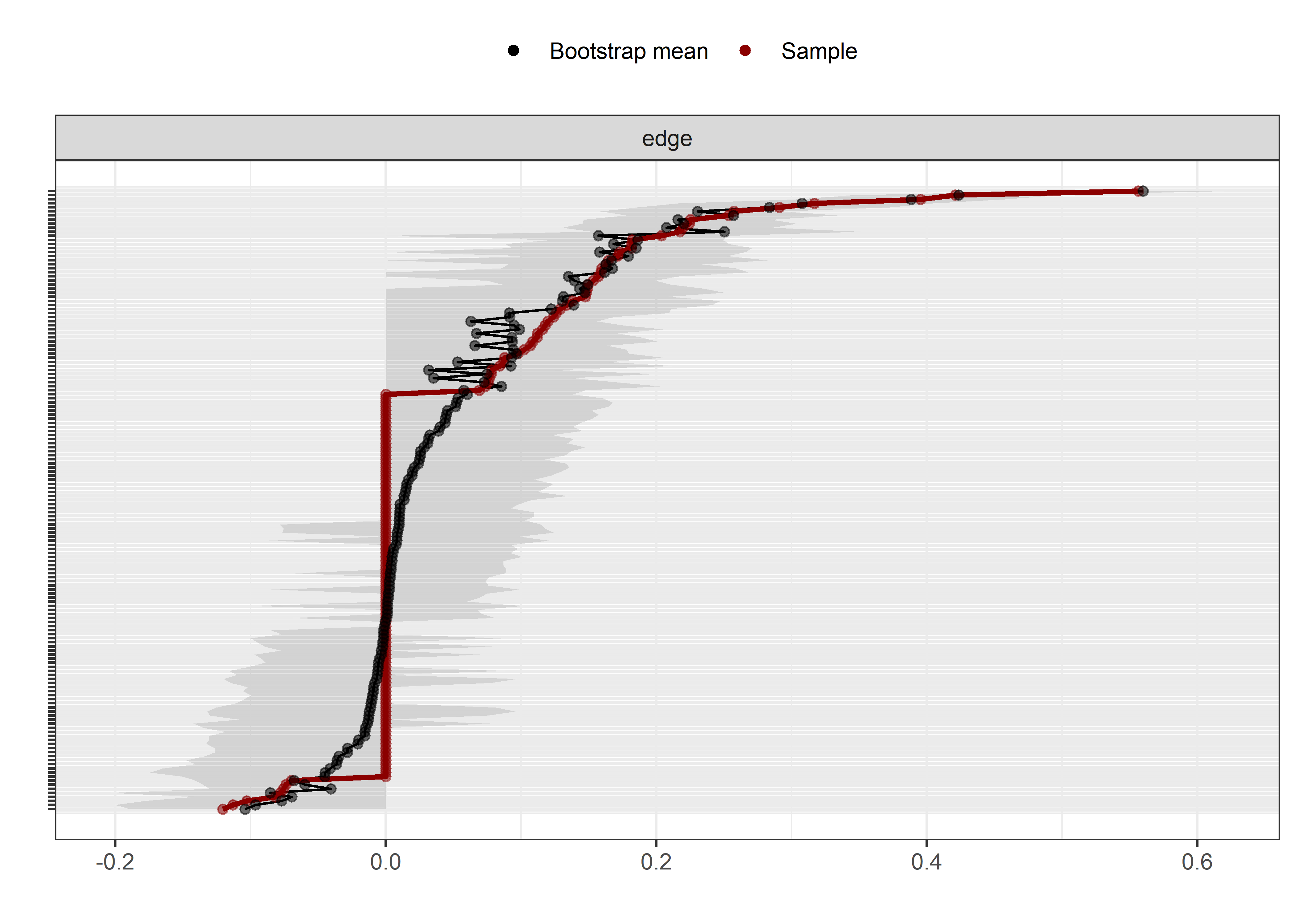
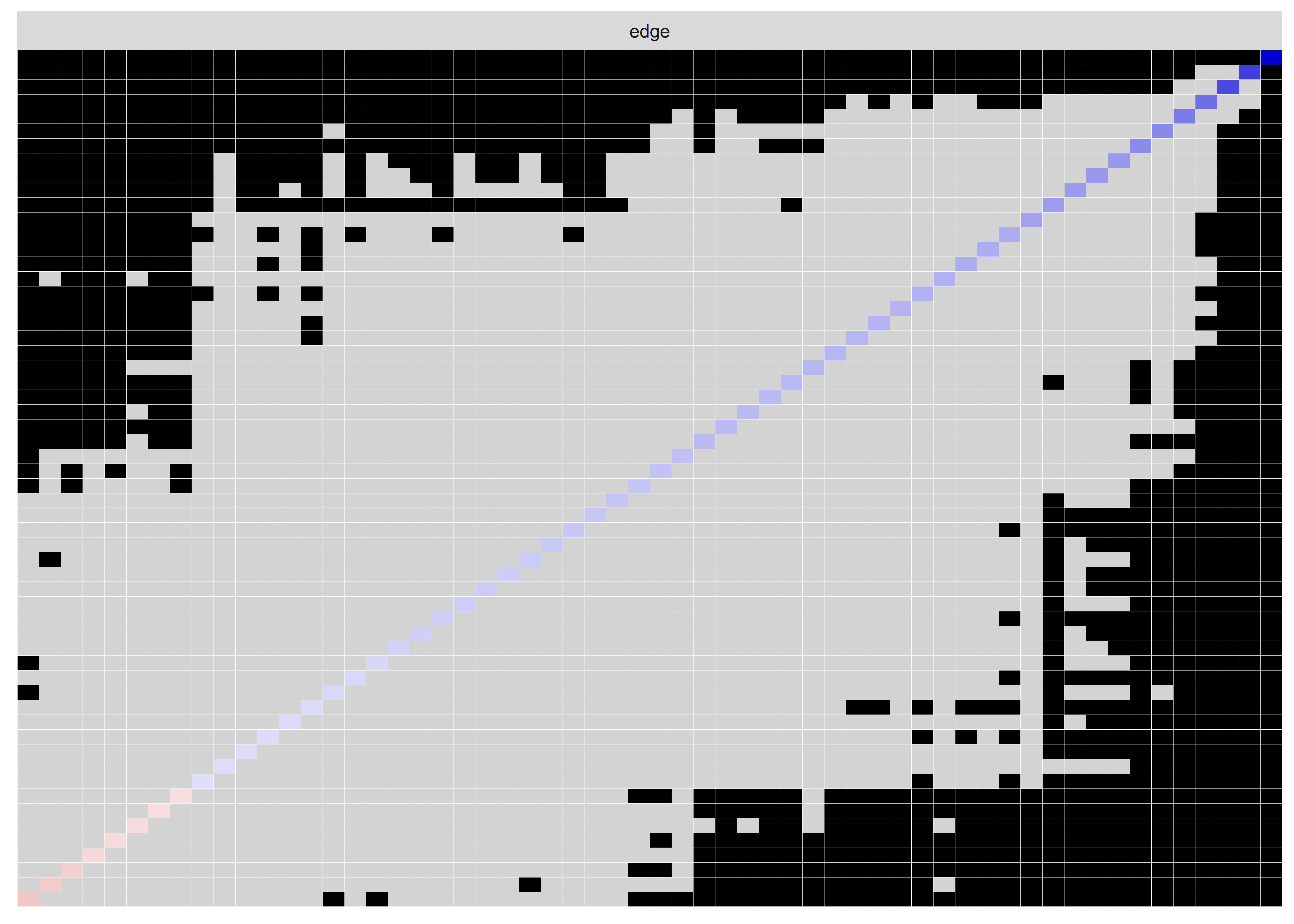
# bootnet_centrality_stability_onlyCombinedBctsIsing <- bootnet::bootnet(onlyCombinedBctsIsing, stepwise = FALSE, nBoots=1000,nCores=8, type="case")
# save(bootnet_centrality_stability_onlyCombinedBctsIsing, file = "./Rdata_files/bootnet_centrality_stability_onlyCombinedBctsIsing.Rdata")
# load("./Rdata_files/bootnet_centrality_stability_onlyCombinedBctsIsing.Rdata")
#
# plot(bootnet_centrality_stability_onlyCombinedBctsIsing)
# plot(bootnet_centrality_stability_onlyCombinedBctsIsing, perNode=T, "strength")
#
# bootnet::corStability(bootnet_centrality_stability_onlyCombinedBctsIsing)
GGM BCTs & motivation
The pie on nodes represents the median, as proportion of the theoretical maximum value (i.e. highest value on the questionnaire scale).
library(corrgram)

nItems <- 19

bctdf <- df %>% dplyr::select(id,
  intervention,
  group,
  school,
  girl,
  'Autonomous' = PA_autonomous_T1,
  'Controlled' = PA_controlled_T1,
  'goal setting' = PA_agreementDependentBCT_01_T1,
  'own plan' = PA_agreementDependentBCT_02_T1,
  'plan by other' = PA_agreementDependentBCT_03_T1,
  'reminder of plan' = PA_agreementDependentBCT_04_T1,
  'subgoals' = PA_agreementDependentBCT_05_T1,
  'trying new PA' = PA_agreementDependentBCT_06_T1,
  'barrier identification' = PA_agreementDependentBCT_07_T1,
  'problem solving' = PA_agreementDependentBCT_08_T1,
  'PA identity reflection' = PA_agreementDependentBCT_09_T1,
  'aligning PA with life values' = PA_agreementDependentBCT_10_T1,
  'remind of PA benefits' = PA_frequencyDependentBCT_01_T1,
  'self-monitor (paper)' = PA_frequencyDependentBCT_02_T1,
  'self-monitor (app)' = PA_frequencyDependentBCT_03_T1,
#  'memory cues' = PA_frequencyDependentBCT_04_T1,
  'goal review' = PA_frequencyDependentBCT_05_T1,
  'personal relevance reflection' = PA_frequencyDependentBCT_06_T1,
  'environmental changes (home)' = PA_frequencyDependentBCT_07_T1,
  'social support' = PA_frequencyDependentBCT_08_T1,
  'failure contemplated' = PA_frequencyDependentBCT_09_T1) %>%
  rowwise() %>%
  mutate(
  #'has plan' = mean(c(`own plan`, `plan by other`), na.rm = TRUE),
  'self-monitor' = mean(c(`self-monitor (paper)`, `self-monitor (app)`), na.rm = TRUE)) %>%
  dplyr::select(-`self-monitor (paper)`, -`self-monitor (app)`) %>%
  mutate_all(as.numeric)

# Network for all participants

S.total <- bctdf %>% dplyr::select(`Autonomous`:ncol(bctdf))
nwBCT <- bootnet::estimateNetwork(S.total, default="ggmModSelect")

# Plot correlations (minmax crowds the diagonal as it plots the minimum and maximum values for each variable).
labs <- colnames(S.total)
corrgram::corrgram(S.total,
         cor.method = "spearman",
         # diag.panel=panel.minmax,
         # lower.panel=panel.shade,
         # lower.panel=panel.ellipse,
         # lower.panel=panel.cor,
         upper.panel=corrgram::panel.conf,
         lower.panel=corrgram::panel.conf,
         outer.labels=list(
           bottom=list(labels=labs,cex=.75, srt=60),
           left=list(labels=labs,cex=.75, srt=30))
         )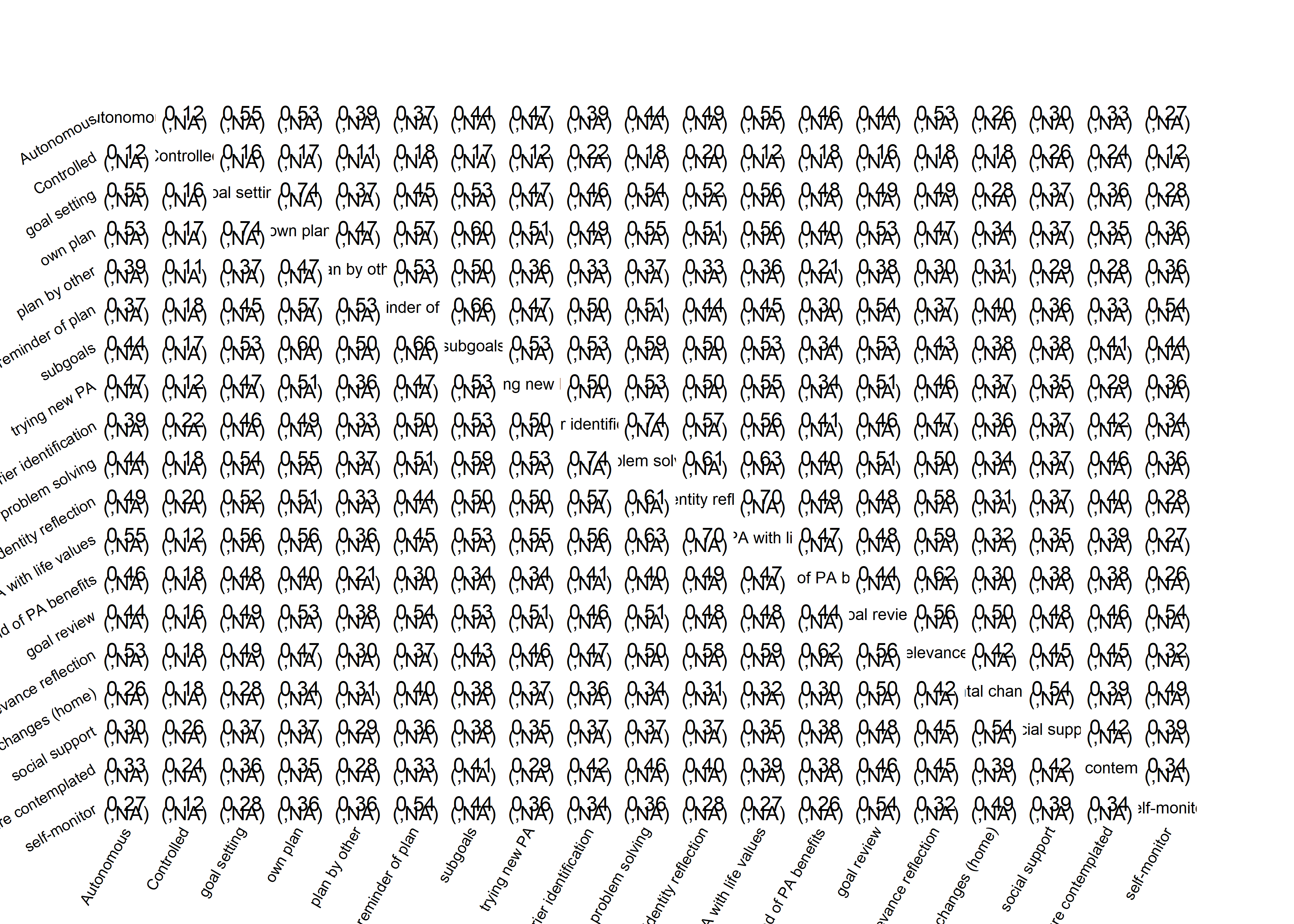
# Create means for filling nodes
piefill <- S.total %>%
  dplyr::select(-Autonomous, -Controlled) %>%
  data.frame() %>%
  summarise_all(funs(mean(., na.rm = TRUE) / 6))

piefill$Autonomous <- median(S.total$Autonomous, na.rm = TRUE) / 5
piefill$Controlled <- median(S.total$Controlled, na.rm = TRUE) / 5

piefill <- piefill %>% select(Autonomous, Controlled, everything())

# Plot network
plot(nwBCT, layout = "spring", label.scale = FALSE, title = "GGM: BCTs & motivation", label.cex = 0.75,
     pie = piefill,
     color = "skyblue",
     pieBorder = 1)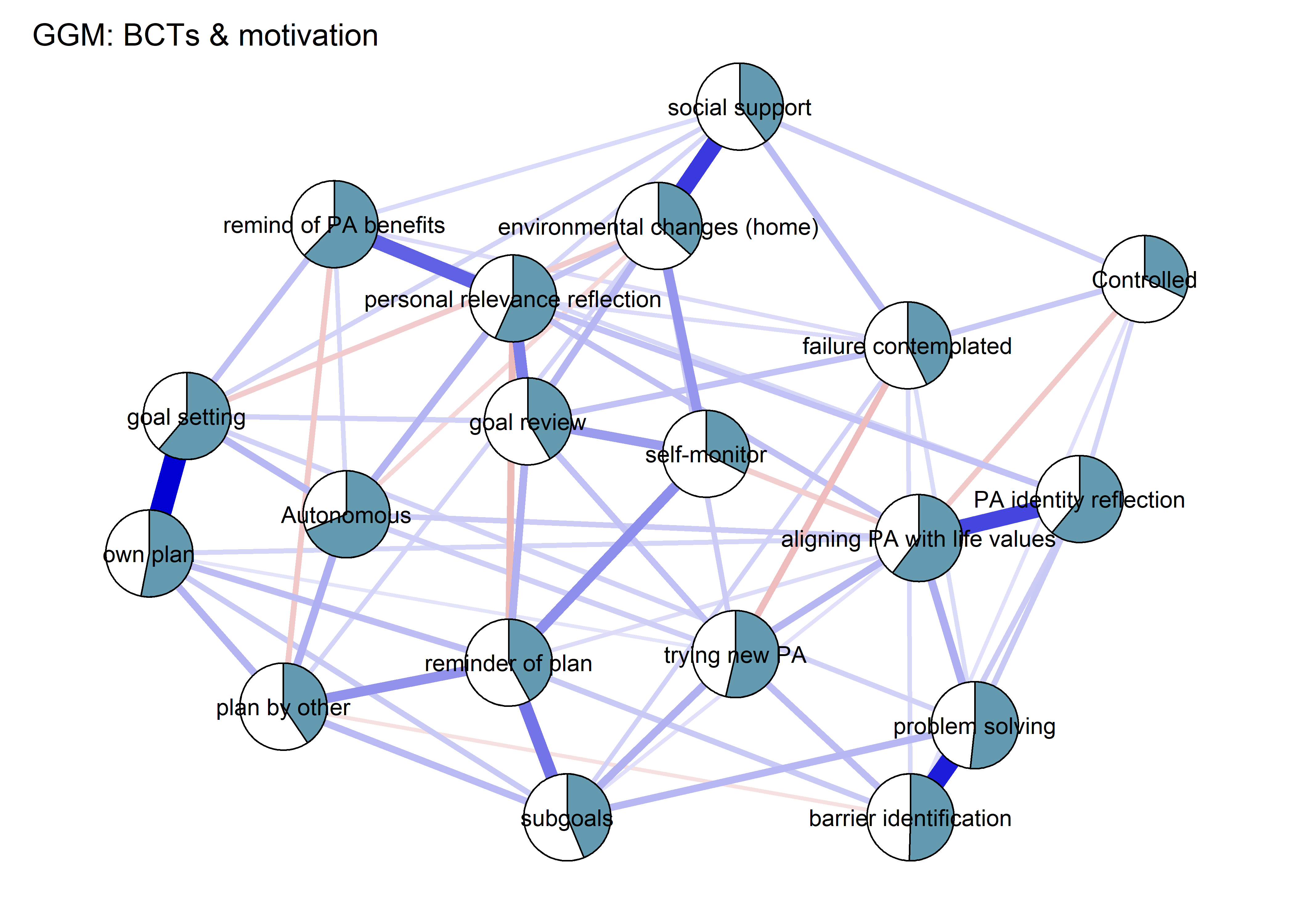
Network after combining goal setting and own planning, as well as barrier identification and problem solving:
# Combine items further:
bctdf2 <- bctdf %>% rowwise %>%
  dplyr::mutate('goals and plans' = mean(c(`goal setting`, `own plan`), na.rm = TRUE)) %>%
  dplyr::mutate('barriers identified\nand planned for' = mean(c(`barrier identification`, `problem solving`), na.rm = TRUE)) %>%
  dplyr::select(-`goal setting`, -`own plan`, -`barrier identification`, -`problem solving`)

S.total2 <- bctdf2 %>% dplyr::select(`Autonomous`:ncol(bctdf2))
nwBCT2 <- bootnet::estimateNetwork(S.total2, default="ggmModSelect")

# Create means for filling nodes
piefill2 <- S.total2 %>%
  dplyr::select(-Autonomous, -Controlled) %>%
  data.frame() %>%
  summarise_all(funs(median(., na.rm = TRUE) / 6))

piefill2$Autonomous <- median(S.total$Autonomous, na.rm = TRUE) / 5
piefill2$Controlled <- median(S.total$Controlled, na.rm = TRUE) / 5

piefill2 <- piefill2 %>% select(Autonomous, Controlled, everything())

# Plot network
plot(nwBCT2, layout = "spring", label.scale = FALSE, title = "GGM, BCTs & motivation, items combined", label.cex = 0.75,
     pie = piefill2,
     color = "skyblue",
     pieBorder = 1)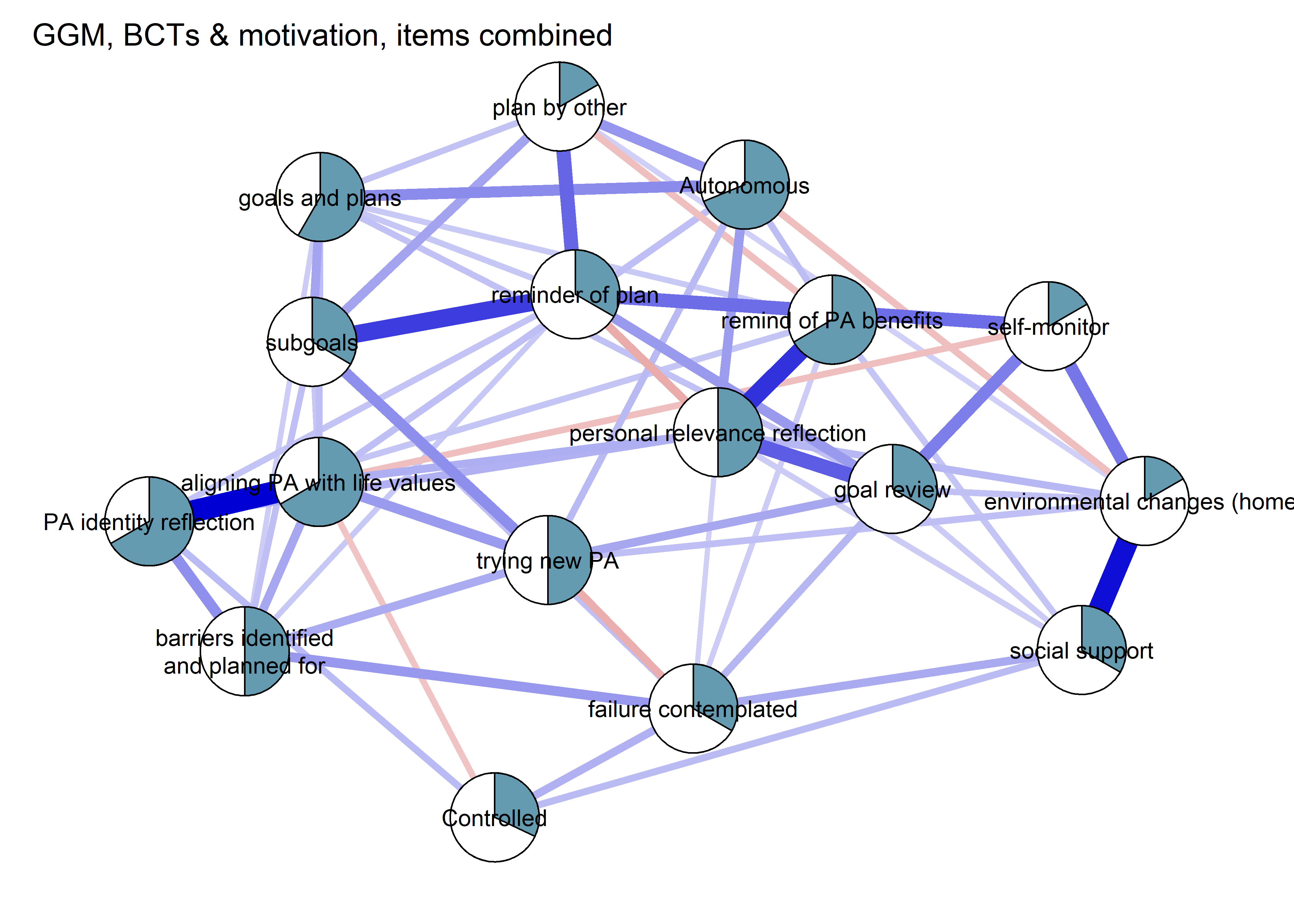
Stability and robustness
Robustness test
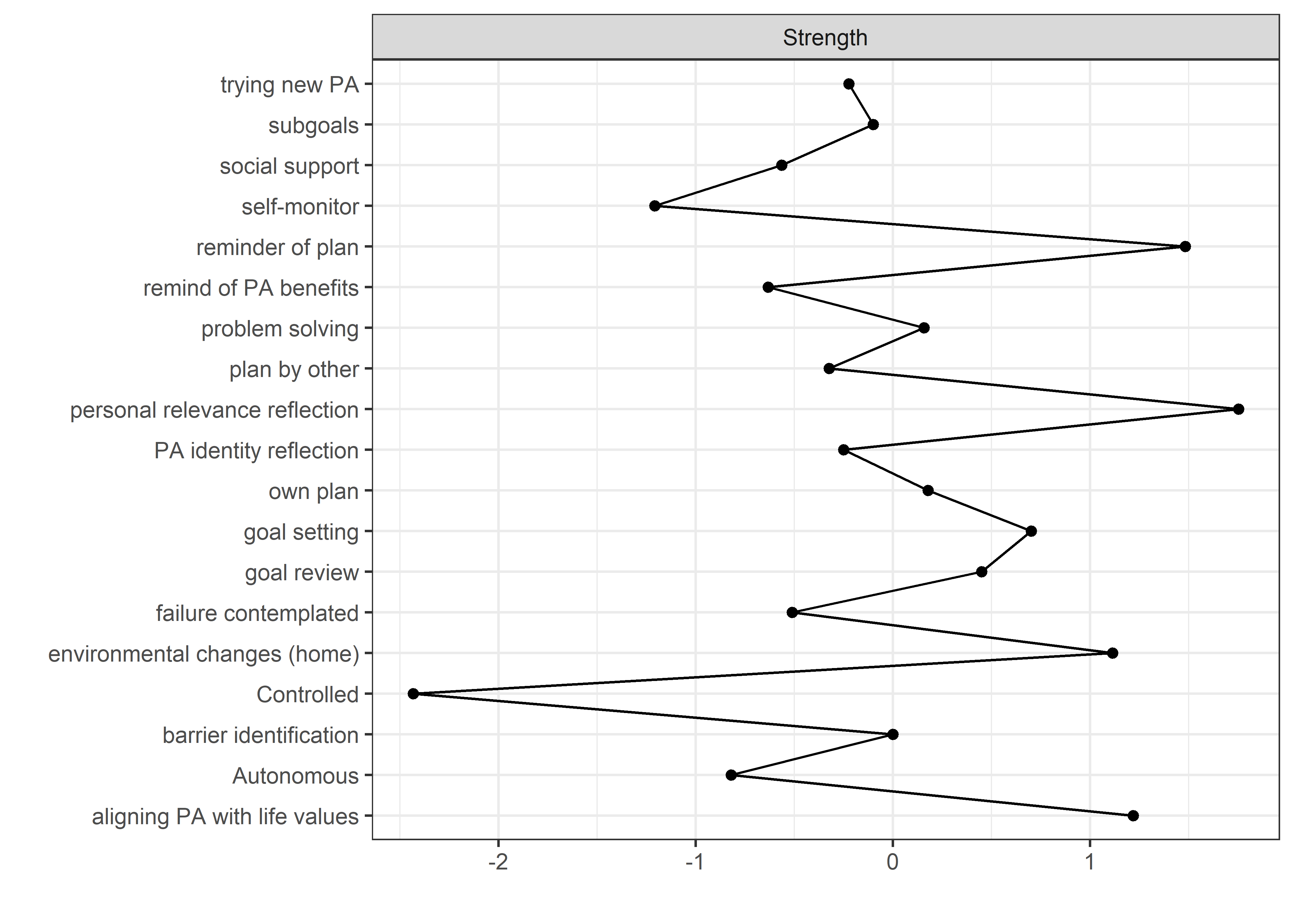
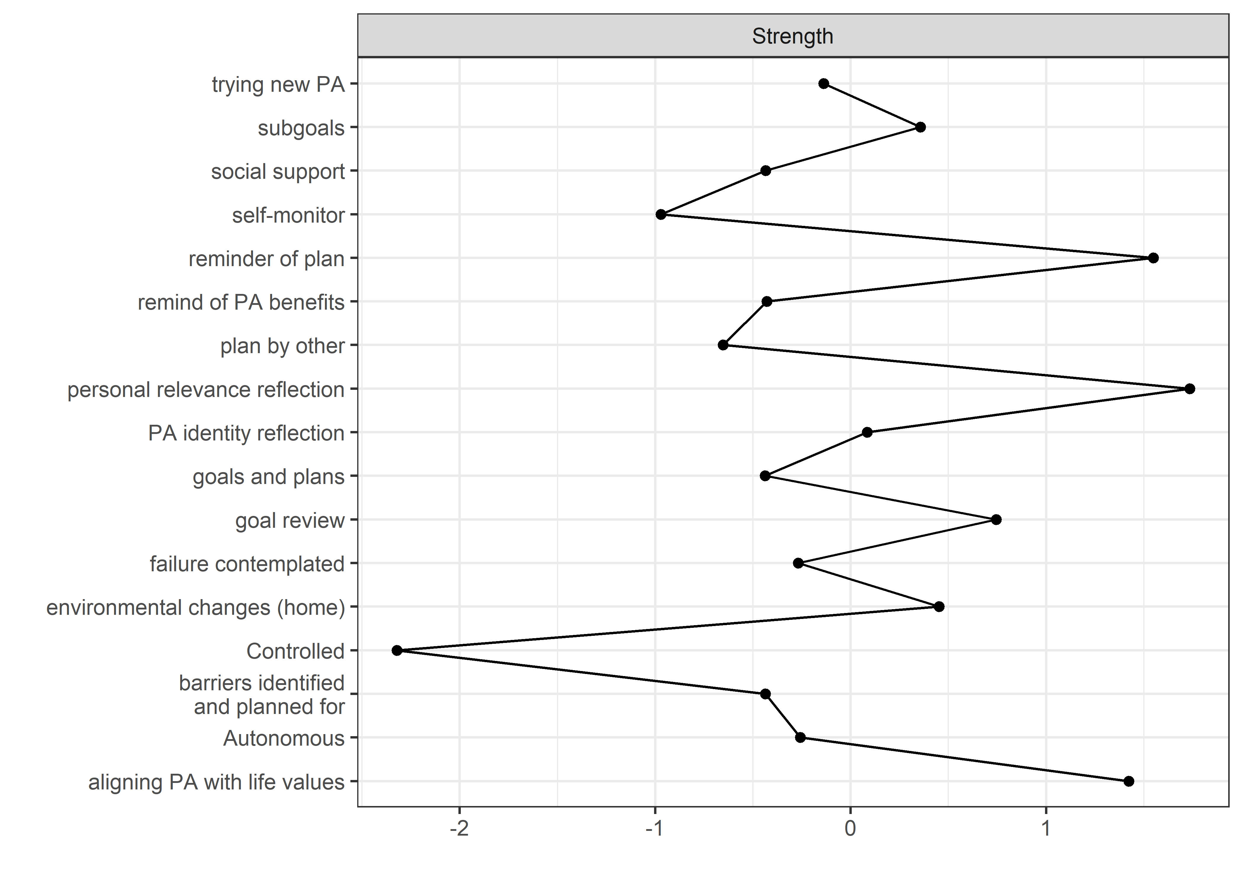
# BCTboot1 <- bootnet::bootnet(nwBCT, stepwise = FALSE, nBoots = 2500)
# BCTboot2 <- bootnet::bootnet(nwBCT2, stepwise = FALSE, nBoots = 2500)
# save(BCTboot1, file = "./Rdata_files/BCTboot1.Rdata")
# save(BCTboot2, file = "./Rdata_files/BCTboot2.Rdata")

load("./Rdata_files/BCTboot1.Rdata")
load("./Rdata_files/BCTboot2.Rdata")

print("Original items:")
## [1] "Original items:"
plot(BCTboot1, labels = FALSE, order = "sample")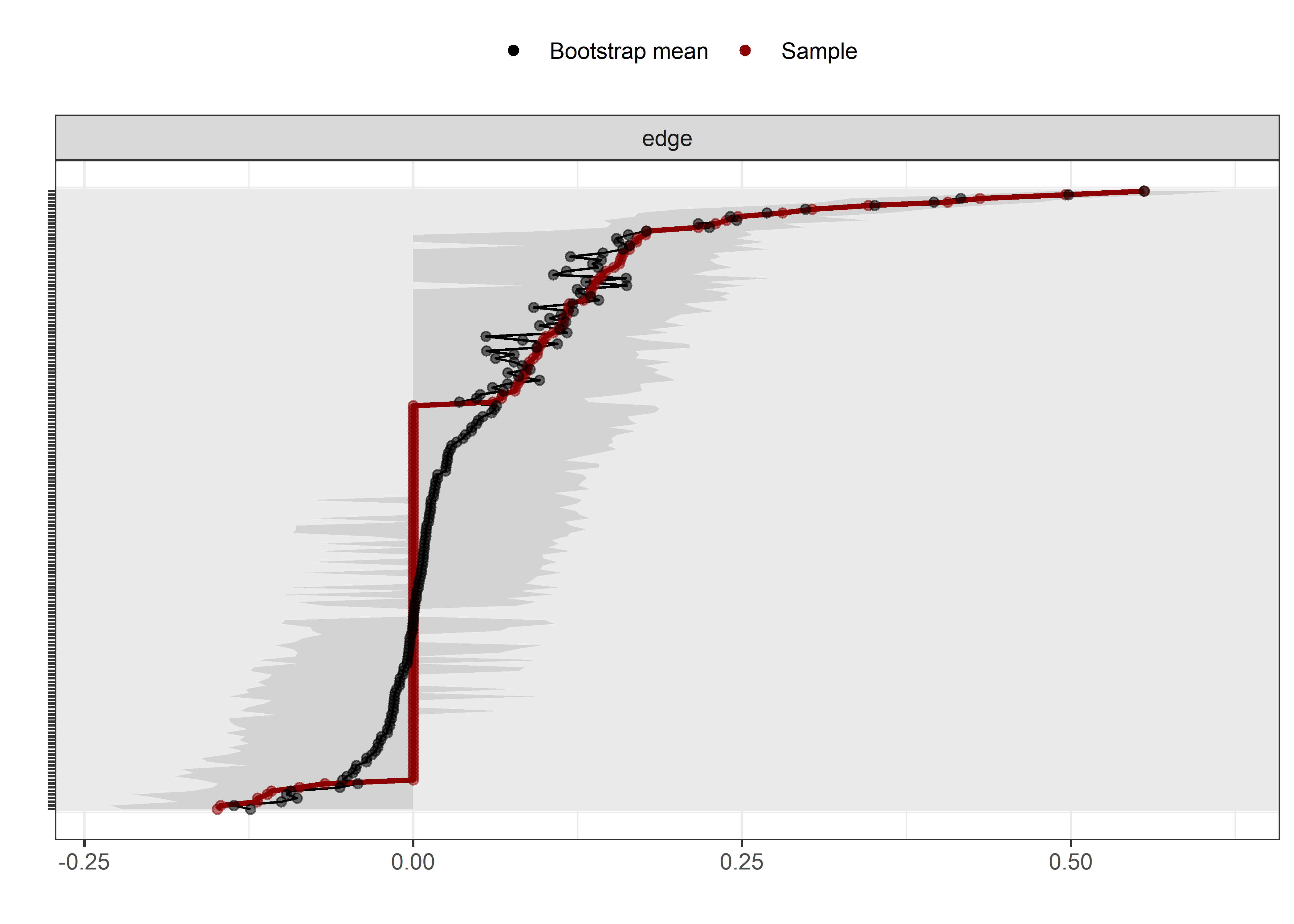
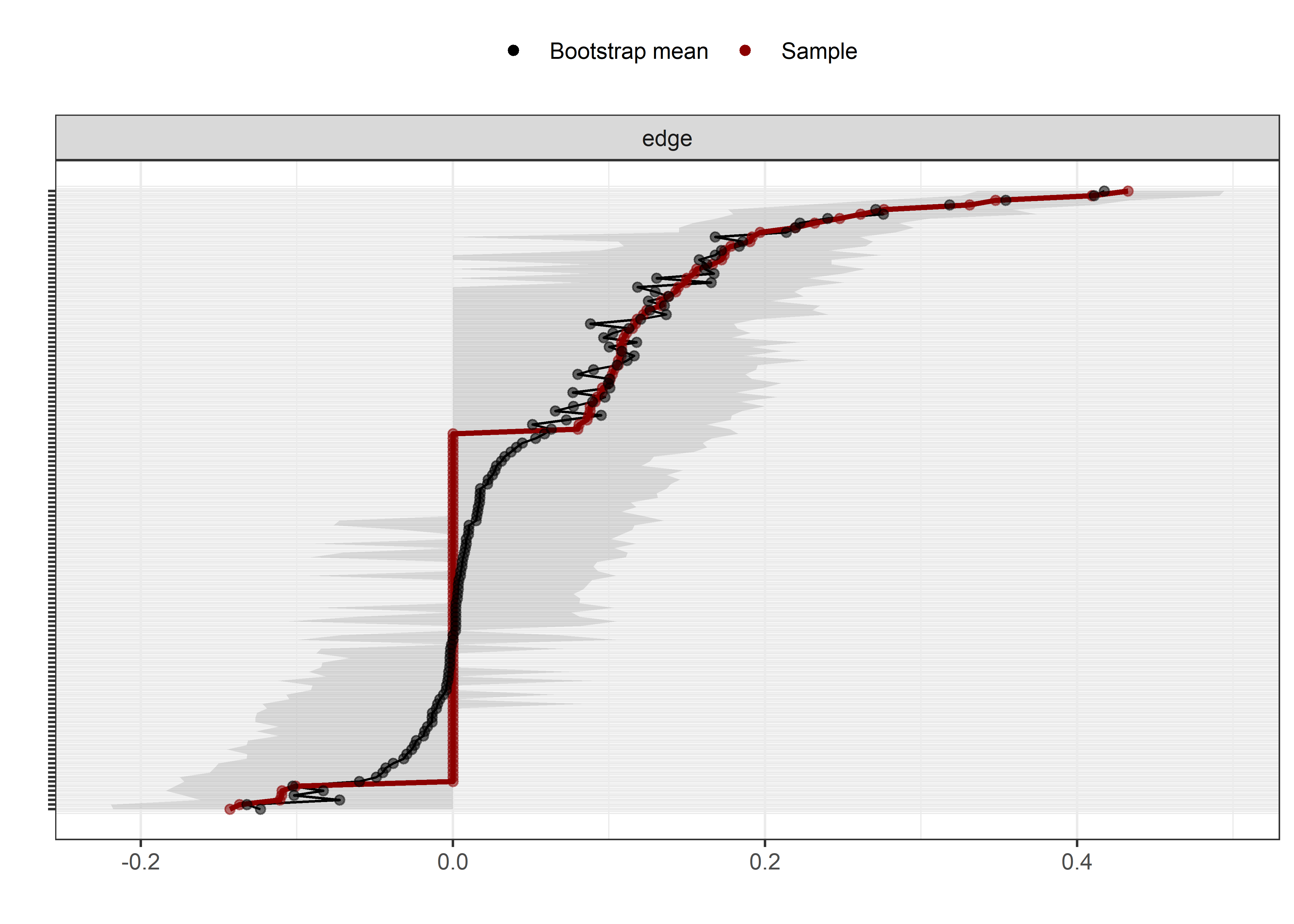
autEdges <- summary(BCTboot1, statistics = "edge", rank = TRUE) %>%
  dplyr::arrange(mean) %>%
  dplyr::filter(stringr::str_detect(node1, 'Autonomous')) %>% # str_detect(id, 'Autonomous|Controlled') for both
  dplyr::filter(!(node2 == 'Controlled')) %>%
  data.frame() %>%
  dplyr::select(CIlower, mean, CIupper, node2)

contEdges <- summary(BCTboot1, statistics = "edge", rank = TRUE) %>%
  dplyr::arrange(mean) %>%
  dplyr::filter(stringr::str_detect(node1, 'Controlled')) %>% # str_detect(id, 'Autonomous|Controlled') for both
  data.frame() %>%
  dplyr::select(CIlower, mean, CIupper, node2)

userfriendlyscience::diamondPlot(autEdges,
            ciCols = c("CIlower", "mean", "CIupper"),
            color = viridis::viridis(2, end = 0.8)[1],
            alpha = 0.3,
            yLabels = autEdges$node2,
            fixedSize = 0.3,
            xlab = NULL) +
  userfriendlyscience::diamondPlot(contEdges,
              ciCols = c("CIlower", "mean", "CIupper"),
              color = viridis::viridis(2, end = 0.8)[2],
              alpha = 0.3,
              yLabels = autEdges$node2,
              fixedSize = 0.3,
              xlab = NULL,
              returnLayerOnly = TRUE) +
  geom_rect(aes(xmin=Inf, xmax=Inf, ymin=Inf, ymax=Inf, fill = "Controlled"),
            colour=NA, alpha=0.05) + # Create invisible rectangle for legend
  geom_rect(aes(xmin=Inf, xmax=Inf, ymin=Inf, ymax=Inf, fill = "Autonomous"),
            colour=NA, alpha=0.05) + # Create invisible rectangle for legend
  scale_fill_manual('Connected node',
                      values = viridis::viridis(2, end = 0.8)[1:2],
                      guide = guide_legend(override.aes = list(alpha = 1))) +
  ggtitle("Relative strengths of edges containing autonomous \nor controlled motivation (model with all items)")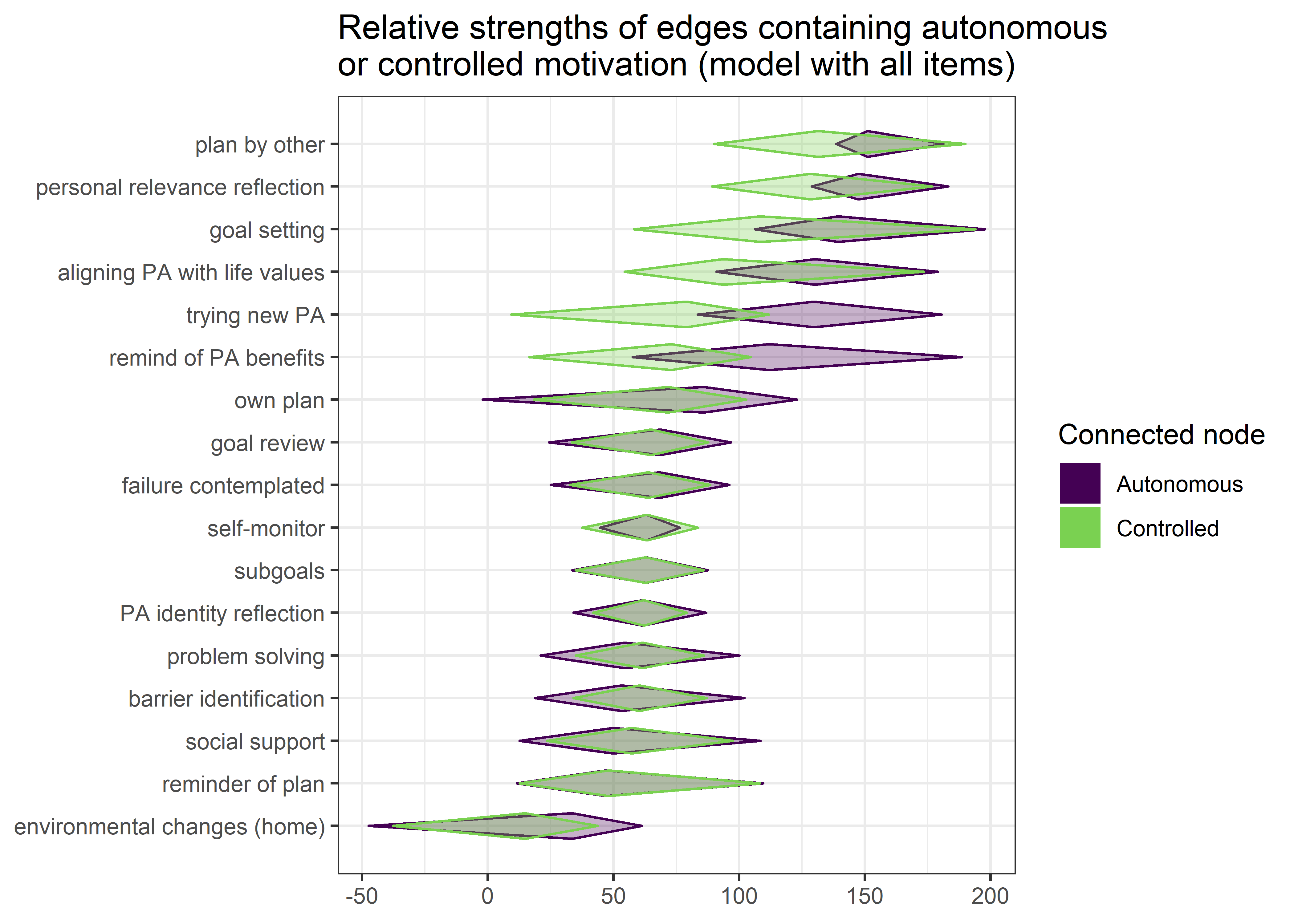
# Combined items

autEdges <- summary(BCTboot2, statistics = "edge", rank = TRUE) %>%
  dplyr::arrange(mean) %>%
  dplyr::filter(stringr::str_detect(node1, 'Autonomous')) %>% # str_detect(id, 'Autonomous|Controlled') for both
  dplyr::filter(!(node2 == 'Controlled')) %>%
  data.frame() %>%
  dplyr::select(CIlower, mean, CIupper, node2)

contEdges <- summary(BCTboot2, statistics = "edge", rank = TRUE) %>%
  dplyr::arrange(mean) %>%
  dplyr::filter(stringr::str_detect(node1, 'Controlled')) %>% # str_detect(id, 'Autonomous|Controlled') for both
  data.frame() %>%
  dplyr::select(CIlower, mean, CIupper, node2)

userfriendlyscience::diamondPlot(autEdges,
            ciCols = c("CIlower", "mean", "CIupper"),
            color = viridis::viridis(2, end = 0.8)[1],
            alpha = 0.3,
            yLabels = autEdges$node2,
            fixedSize = 0.3,
            xlab = NULL) +
  userfriendlyscience::diamondPlot(contEdges,
              ciCols = c("CIlower", "mean", "CIupper"),
              color = viridis::viridis(2, end = 0.8)[2],
              alpha = 0.3,
              yLabels = autEdges$node2,
              fixedSize = 0.3,
              xlab = NULL,
              returnLayerOnly = TRUE) +
  geom_rect(aes(xmin=Inf, xmax=Inf, ymin=Inf, ymax=Inf, fill = "Controlled"),
            colour=NA, alpha=0.05) + # Create invisible rectangle for legend
  geom_rect(aes(xmin=Inf, xmax=Inf, ymin=Inf, ymax=Inf, fill = "Autonomous"),
            colour=NA, alpha=0.05) + # Create invisible rectangle for legend
  scale_fill_manual('Connected node',
                      values = viridis::viridis(2, end = 0.8)[1:2],
                      guide = guide_legend(override.aes = list(alpha = 1))) +
  ggtitle("Relative strengths of edges containing autonomous \nor controlled motivation (model with combined items)")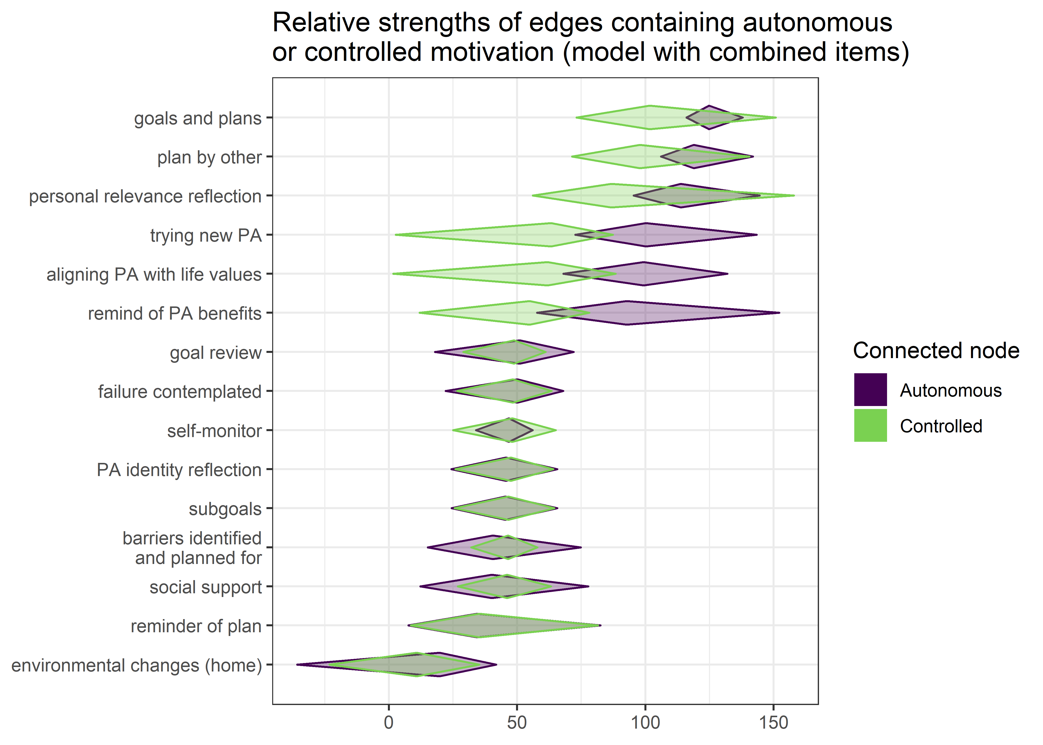
# summary(BCTboot1, statistics = "edge", rank = TRUE) %>%
#   dplyr::arrange(mean) %>%
#   dplyr::filter(stringr::str_detect(id, 'Controlled')) %>%
#   data.frame() %>%
#   dplyr::select(CIlower, mean, CIupper, id) %>%
#   userfriendlyscience::diamondPlot(ciCols = c("CIlower", "mean", "CIupper"), ylabels = id)
Add accelerometer-measured MVPA
nItems_PA <- 20

bctdf_PA <- df %>% dplyr::select(id,
  intervention,
  group,
  school,
  girl,
  'MVPA' = mvpaAccelerometer_T1,
  'Autonomous' = PA_autonomous_T1,
  'Controlled' = PA_controlled_T1,
  'goal setting' = PA_agreementDependentBCT_01_T1,
  'own plan' = PA_agreementDependentBCT_02_T1,
  'plan by other' = PA_agreementDependentBCT_03_T1,
  'reminder of plan' = PA_agreementDependentBCT_04_T1,
  'subgoals' = PA_agreementDependentBCT_05_T1,
  'trying new PA' = PA_agreementDependentBCT_06_T1,
  'barrier identification' = PA_agreementDependentBCT_07_T1,
  'problem solving' = PA_agreementDependentBCT_08_T1,
  'PA identity reflection' = PA_agreementDependentBCT_09_T1,
  'aligning PA with life values' = PA_agreementDependentBCT_10_T1,
  'remind of PA benefits' = PA_frequencyDependentBCT_01_T1,
  'self-monitor (paper)' = PA_frequencyDependentBCT_02_T1,
  'self-monitor (app)' = PA_frequencyDependentBCT_03_T1,
#  'memory cues' = PA_frequencyDependentBCT_04_T1,
  'goal review' = PA_frequencyDependentBCT_05_T1,
  'personal relevance reflection' = PA_frequencyDependentBCT_06_T1,
  'environmental changes (home)' = PA_frequencyDependentBCT_07_T1,
  'social support' = PA_frequencyDependentBCT_08_T1,
  'failure contemplated' = PA_frequencyDependentBCT_09_T1) %>%
  rowwise() %>%
  mutate(
  #'has plan' = mean(c(`own plan`, `plan by other`), na.rm = TRUE),
  'self-monitor' = mean(c(`self-monitor (paper)`, `self-monitor (app)`), na.rm = TRUE)) %>%
  dplyr::select(-`self-monitor (paper)`, -`self-monitor (app)`) %>%
  mutate_all(as.numeric)

# Network for all participants

S.total_PA <- bctdf_PA %>% dplyr::select(`MVPA`:ncol(bctdf_PA))
nwBCT_PA <- bootnet::estimateNetwork(S.total_PA, default="ggmModSelect")

labs <- colnames(S.total_PA)

# Create means for filling nodes
piefill <- S.total_PA %>%
  dplyr::select(-MVPA, -Autonomous, -Controlled) %>%
  data.frame() %>%
  summarise_all(funs(median(., na.rm = TRUE) / 6))

piefill$MVPA <- median(S.total_PA$MVPA, na.rm = TRUE) / (60*24)
piefill$Autonomous <- median(S.total_PA$Autonomous, na.rm = TRUE) / 5
piefill$Controlled <- median(S.total_PA$Controlled, na.rm = TRUE) / 5

piefill <- piefill %>% dplyr::select(MVPA, Autonomous, Controlled, everything())

# Plot network
plot(nwBCT_PA, layout = "spring", label.scale = FALSE, title = "GGM: Accelerometer-MVPA, BCTs & motivation (all items)", label.cex = 0.75,
     pie = piefill,
     color = "skyblue",
     pieBorder = 1)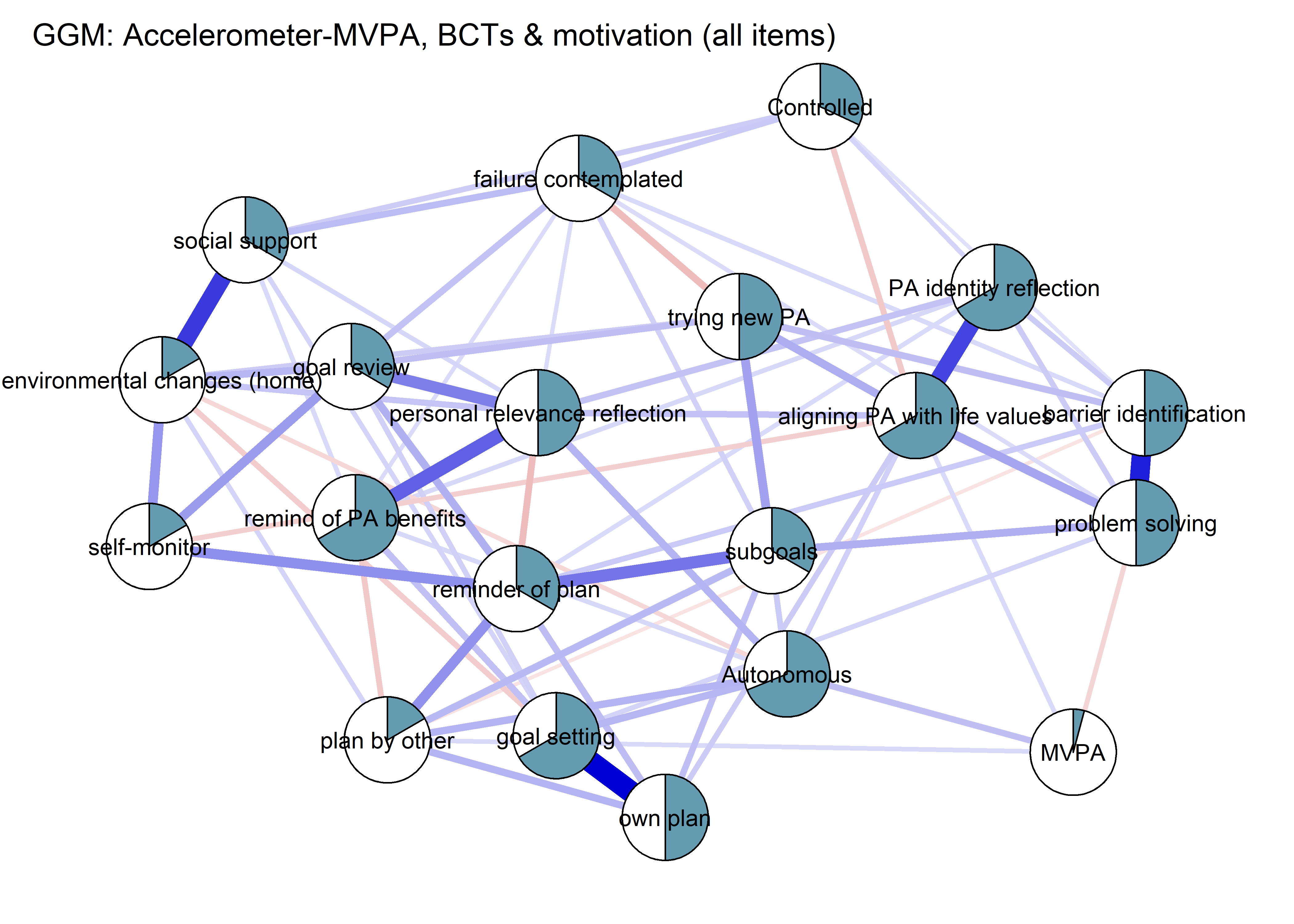
# Combine items further:
bctdf_PA2 <- bctdf_PA %>% rowwise %>%
  mutate('goals and plans' = mean(c(`goal setting`, `own plan`), na.rm = TRUE)) %>%
  mutate('barriers identified\nand planned for' = mean(c(`barrier identification`, `problem solving`), na.rm = TRUE)) %>%
  dplyr::select(-`goal setting`, -`own plan`, -`barrier identification`, -`problem solving`) %>%
  data.frame

S.total_PA2 <- bctdf_PA2 %>% dplyr::select(MVPA:ncol(bctdf_PA2))
nwBCT_PA2 <- bootnet::estimateNetwork(S.total_PA2, default="ggmModSelect")

# Create means for filling nodes
piefill_PA2 <- S.total_PA2 %>%
  dplyr::select(-MVPA, -Autonomous, -Controlled) %>%
  data.frame() %>%
  summarise_all(funs(median(., na.rm = TRUE) / 6))

piefill_PA2$MVPA <- median(S.total_PA2$MVPA, na.rm = TRUE) / (60*24)
piefill_PA2$Autonomous <- median(S.total_PA2$Autonomous, na.rm = TRUE) / 5
piefill_PA2$Controlled <- median(S.total_PA2$Controlled, na.rm = TRUE) / 5

piefill_PA2 <- piefill_PA2 %>% dplyr::select(MVPA, everything())


# Plot network
plot(nwBCT_PA2, layout = "spring", label.scale = FALSE, title = "GGM: Accelerometer-MVPA, BCTs & motivation (combined items)", label.cex = 0.75,
     pie = piefill_PA2,
     color = "skyblue",
     pieBorder = 1)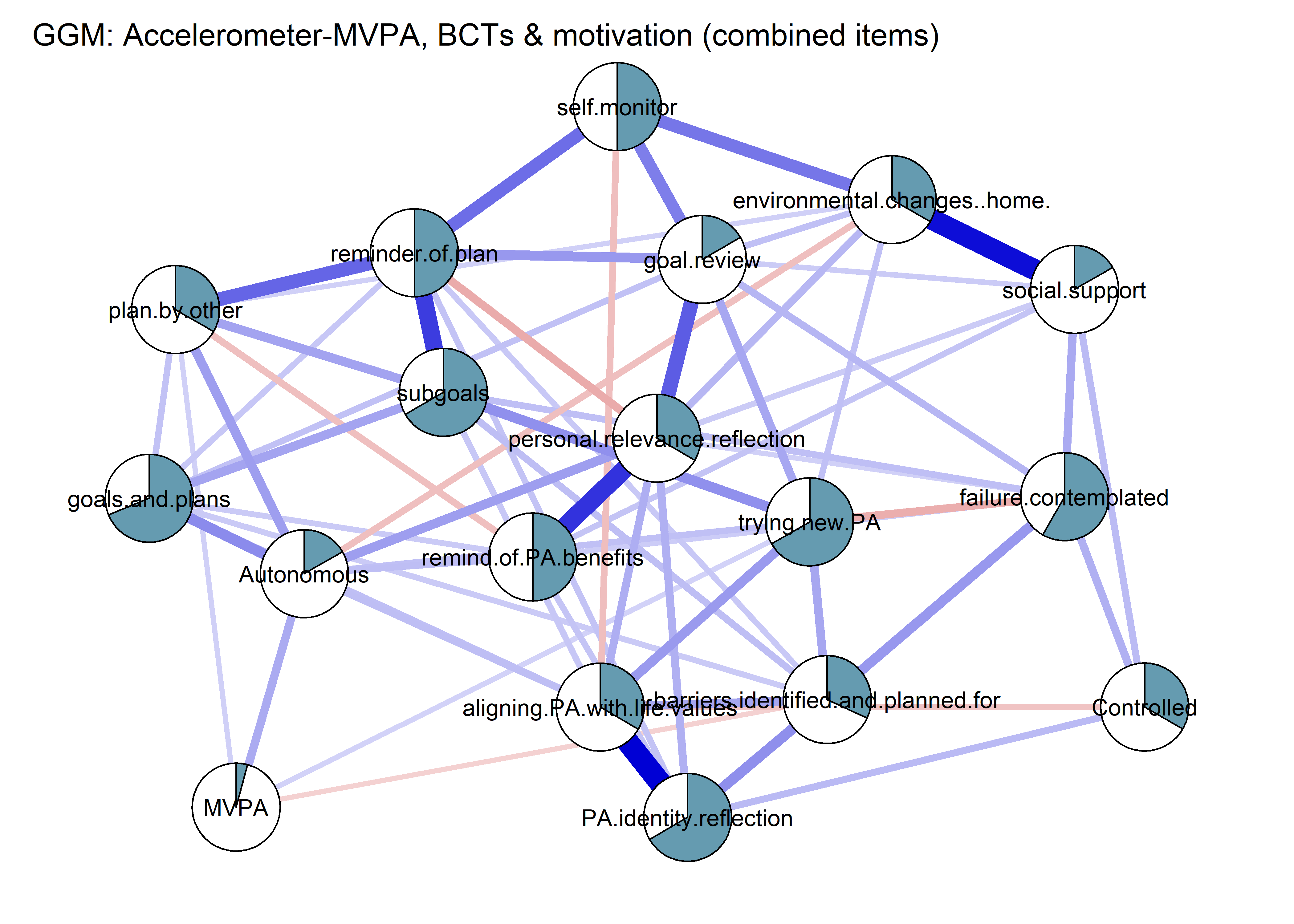
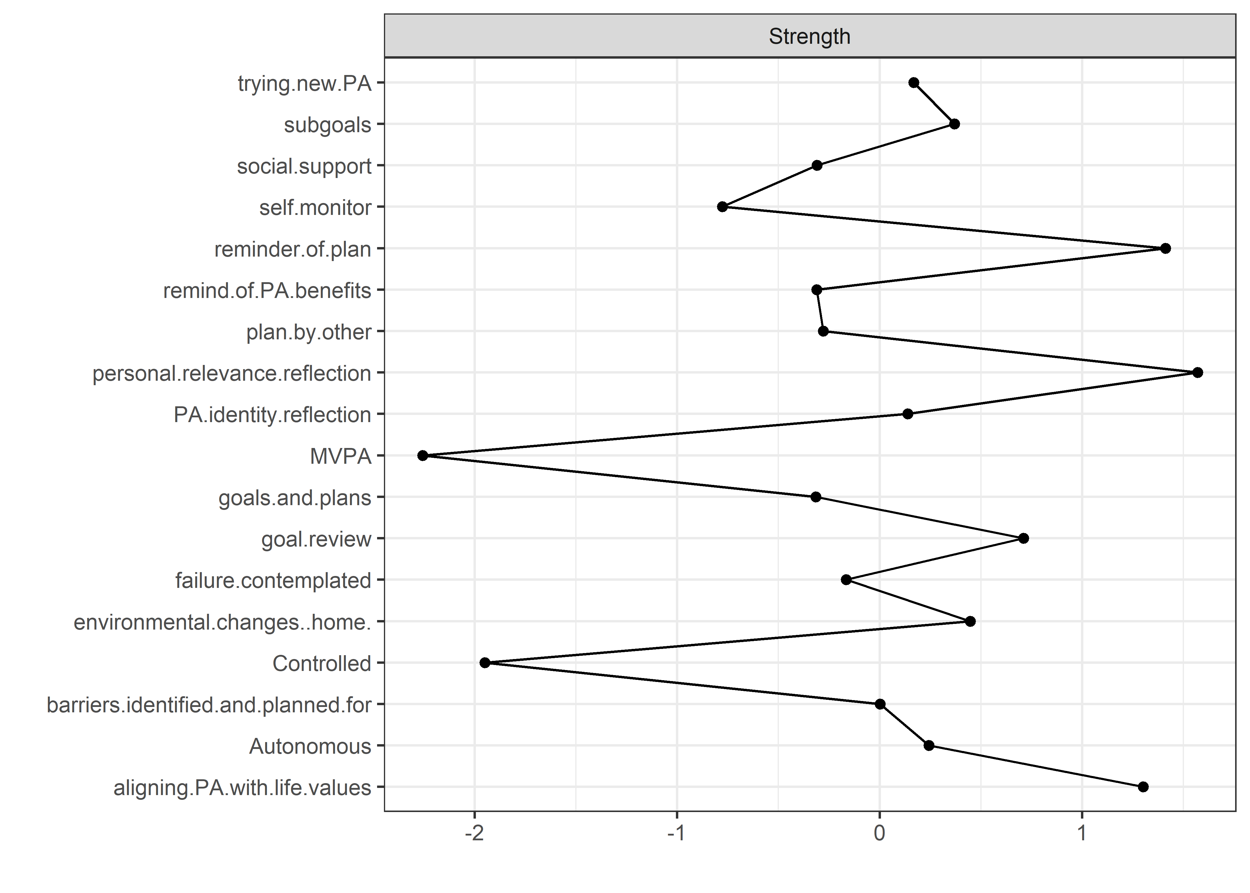
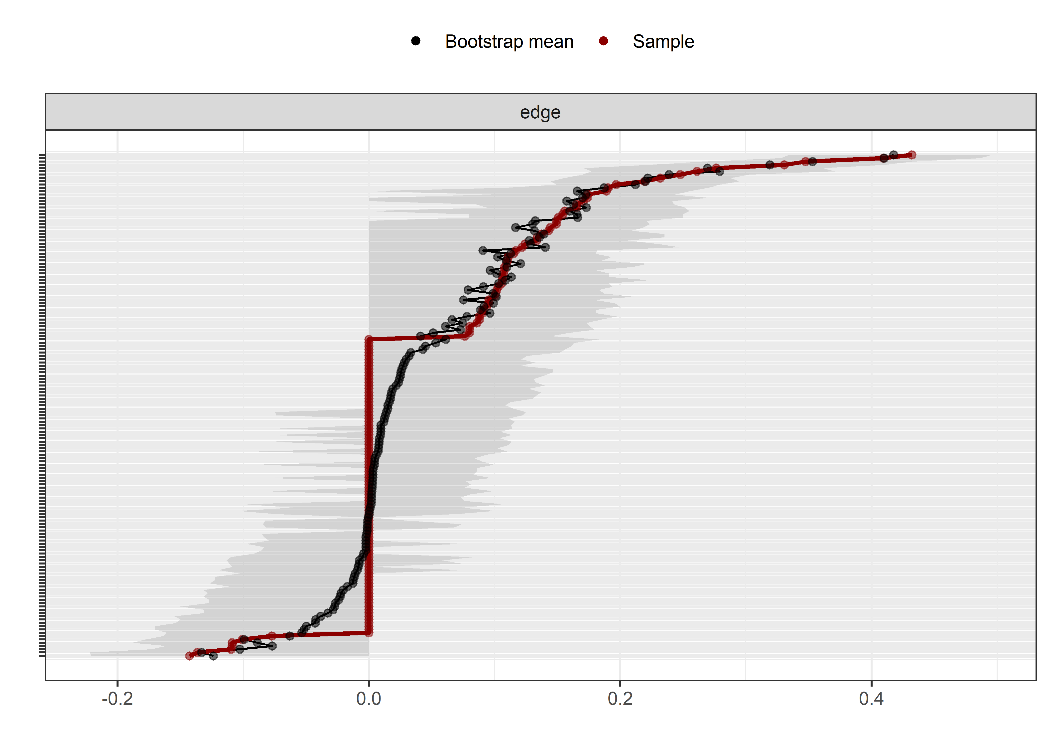
Demonstrating the Ising network
… in PA, autonomous motivation, and top-5 BCTs
Variables are binarised:
* If one reports not using the BCT, they get a zero, otherwise a 1
* If one reports not having done any MVPA during the last week, they get a zero, otherwise a 1
* On the autonomous motivation sum score, if one reports lower agreement than 3 (indicating “sometimes true for me”) on average, they get a zero, otherwise a 1
We include the top 5 BCTs according to their bivariate Spearman correlations with self-reported PA. Self-report instead of accelerometer due to higher sample size and accounting for e.g. gym.
- I have tried out new ways for me to be physically active.
- I have personally made a specific plan (“what, where, how”) to implement my PA.
- I have a PA plan, which has been made by someone else, e.g. my sports club (e.g. a workout schedule).
- I have set PA goals for myself.
- I have broken down larger PA goals to smaller subgoals.
When a person has tried out a new PA way to be physically active, they have almost (because question time scales don’t overlap completely) by definition done MVPA lately. Therefore, we substitute this with:
- I have compared my actualized PA with the PA goal I have set.
top5Bcts_df <- df %>% dplyr::select(
  MVPA = padaysLastweek_T1,
  Autonomous = PA_autonomous_T1,
  'goal review' = PA_frequencyDependentBCT_05_T1,
  'own plan' = PA_agreementDependentBCT_02_T1,
  'plan by other' = PA_agreementDependentBCT_03_T1,
  'goal setting' = PA_agreementDependentBCT_01_T1,
  'subgoals' = PA_agreementDependentBCT_05_T1) %>%
 mutate(
  'MVPA' = ifelse(`MVPA` == 0, 0, 1),
  'Autonomous' = ifelse(`Autonomous` < 3, 0, 1),
  'goal review' = ifelse(`goal review` == 1, 0, 1),
  'own plan' = ifelse(`own plan` == 1, 0, 1),
  'plan by other' = ifelse(`plan by other` == 1, 0, 1),
  'goal setting' = ifelse(`goal setting` == 1, 0, 1),
  'subgoals' = ifelse(`subgoals` == 1, 0, 1))

allMeans <- top5Bcts_df %>%
  summarise_all(funs(mean(., na.rm = TRUE)))

network_all <- bootnet::estimateNetwork(top5Bcts_df, default="IsingFit")
##
  |
  |                                                                 |   0%
  |
  |=========                                                        |  14%
  |
  |===================                                              |  29%
  |
  |============================                                     |  43%
  |
  |=====================================                            |  57%
  |
  |==============================================                   |  71%
  |
  |========================================================         |  86%
  |
  |=================================================================| 100%

graph_cor <- qgraph::qgraph(qgraph::cor_auto(top5Bcts_df), graph = "cor", layout="spring", cut=0,
                  label.scale = FALSE, edge.labels = TRUE, labels = names(top5Bcts_df),
                  pie = allMeans, pieBorder = 1, title = "Bivariate correlations")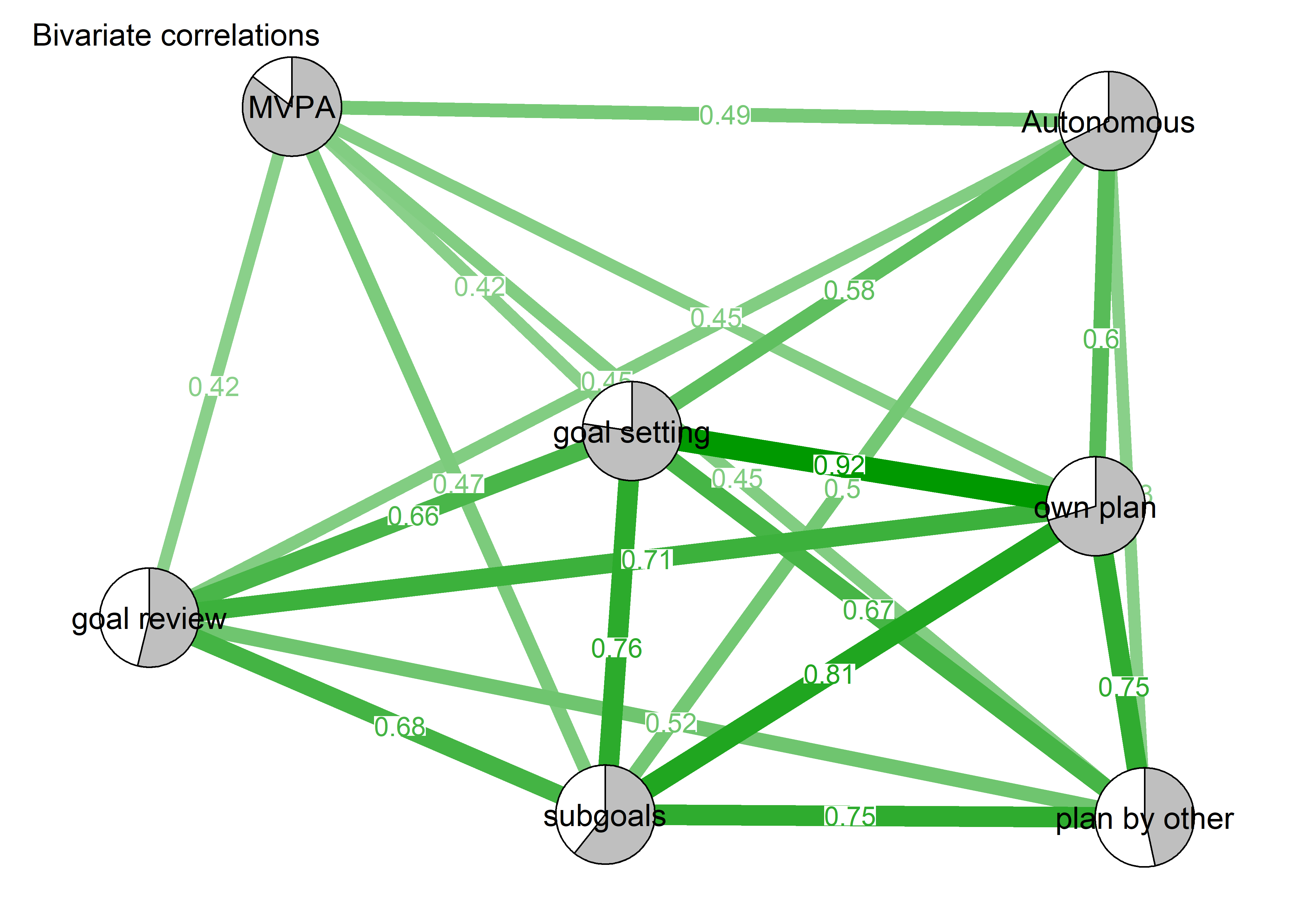
graph_Ising <- plot(network_all, layout="spring", cut=0, label.scale = FALSE,
                  pie = allMeans, pieBorder = 1, title = "Ising model")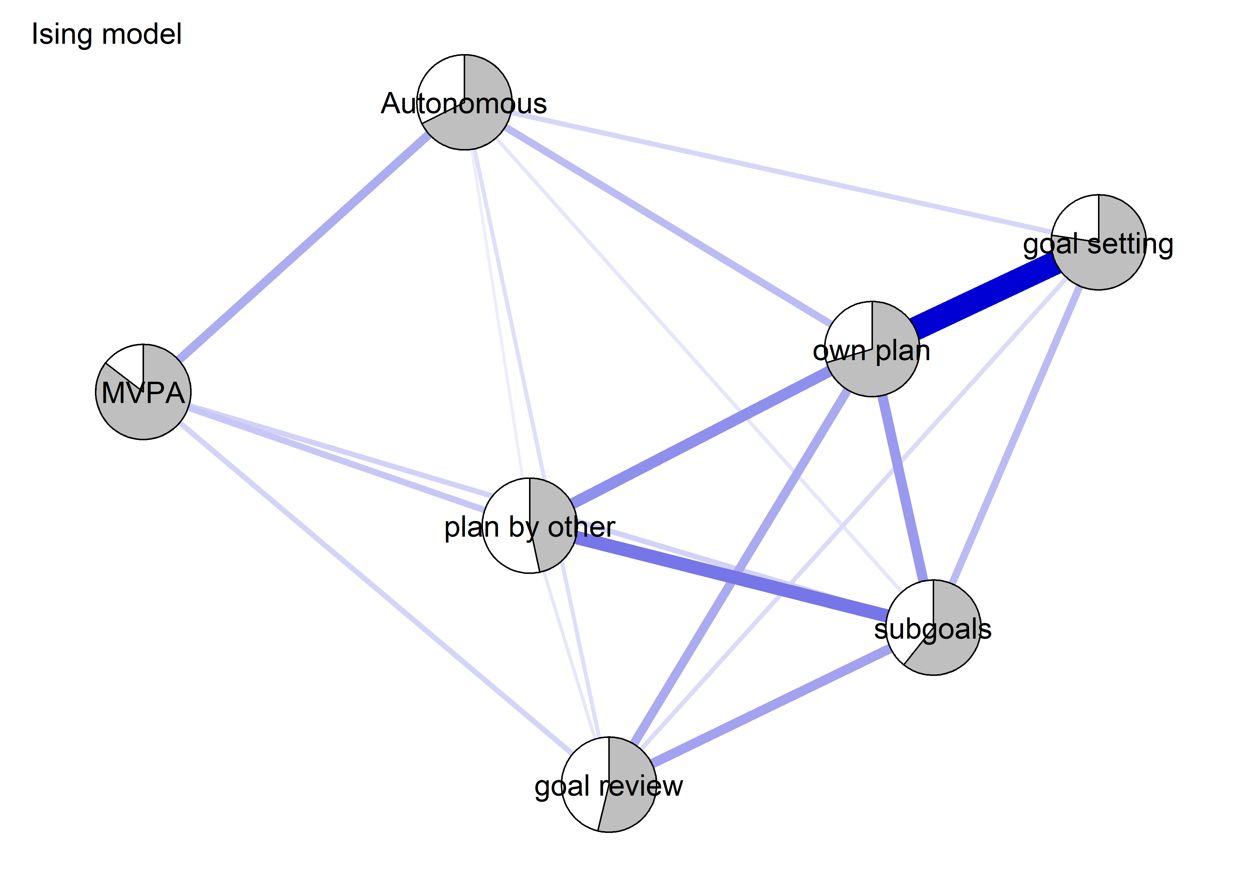
# maxedge <- max(c(graph_Ising$graphAttributes$Graph$maximum,
#                  graph_cor$graphAttributes$Graph$maximum))

L <- qgraph::averageLayout(graph_cor, graph_Ising)

layout(matrix(1:2, nrow = 1, byrow = TRUE))
graph_cor <- qgraph::qgraph(qgraph::cor_auto(top5Bcts_df), graph = "cor", layout=L, cut=0,
                  label.scale = FALSE, edge.labels = TRUE, labels = names(top5Bcts_df), label.cex = 0.8,
                  pie = allMeans, pieBorder = 1, title = "Bivariate correlations")
graph_Ising <- plot(network_all, layout=L, cut=0, label.scale = FALSE,
                  pie = allMeans, pieBorder = 1, title = "Ising model", label.cex = 0.8)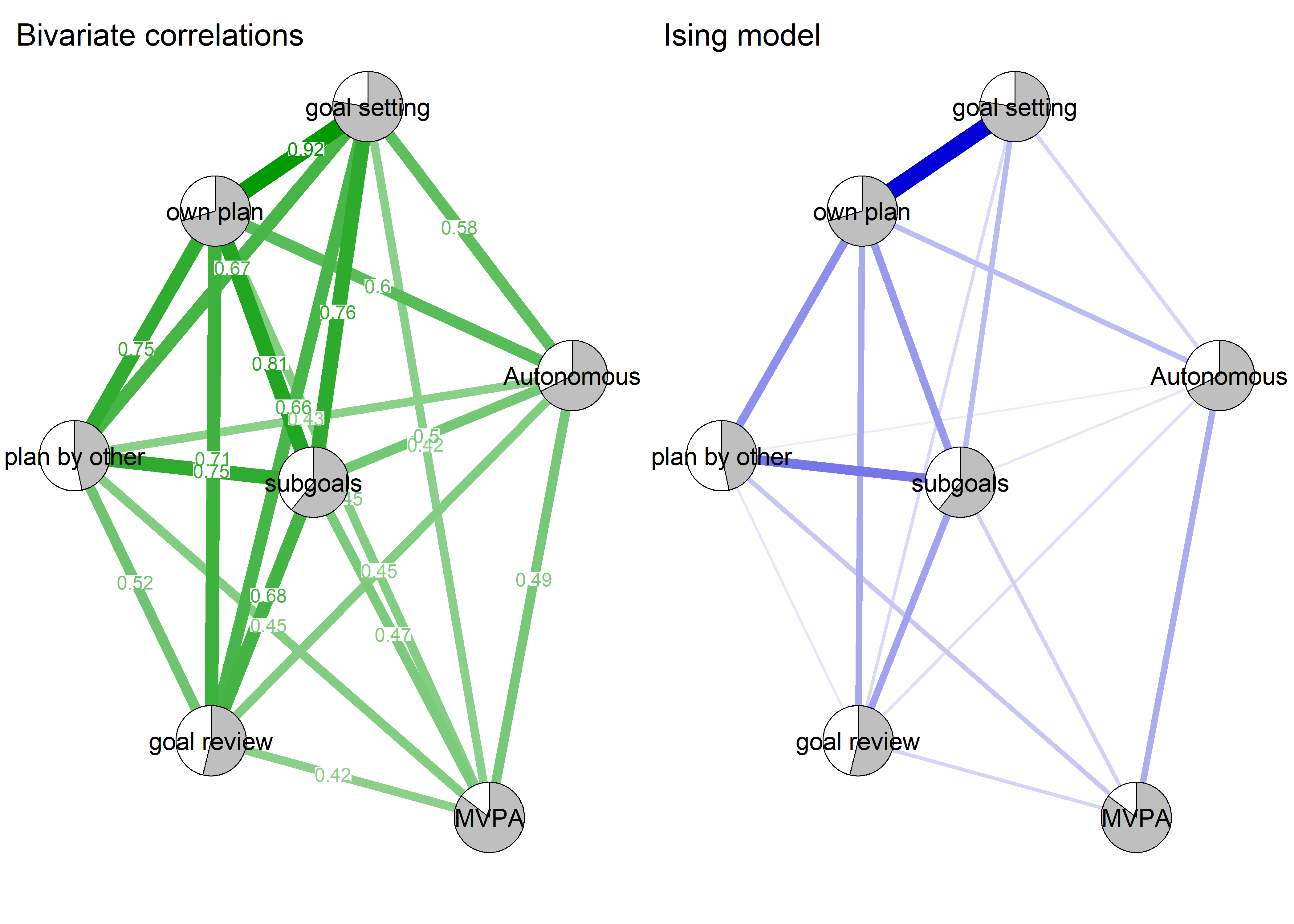
qgraph::flow(graph_Ising,
             "MVPA",
             groups = c("A", "B", rep("C", 5)),
             legend = FALSE,
             title = "",
             vsize = 15,
             label.cex = 1.5,
             colors = viridis::viridis(3),
             label.color = c("white", rep("black", 6)))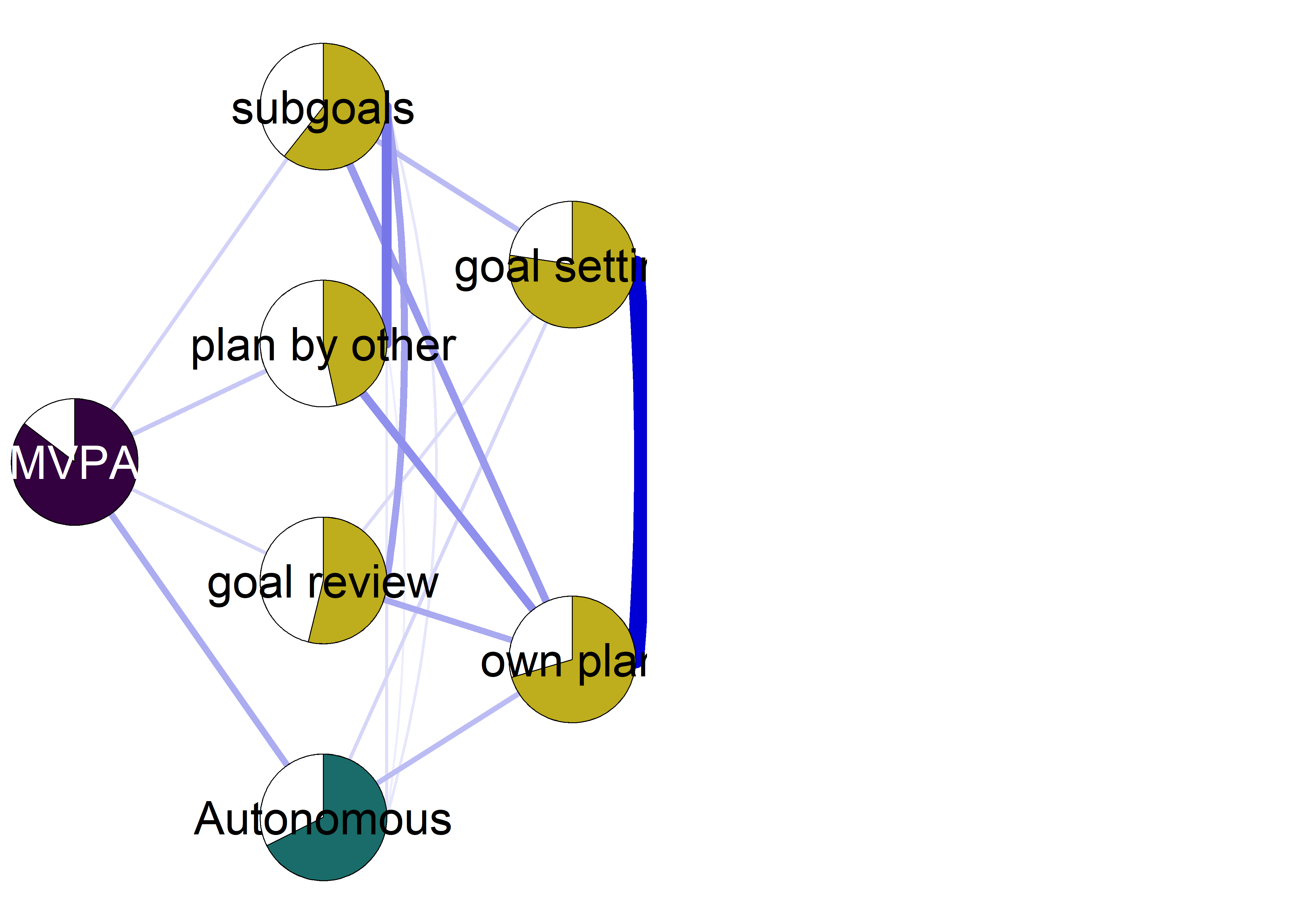
Centrality and stability:
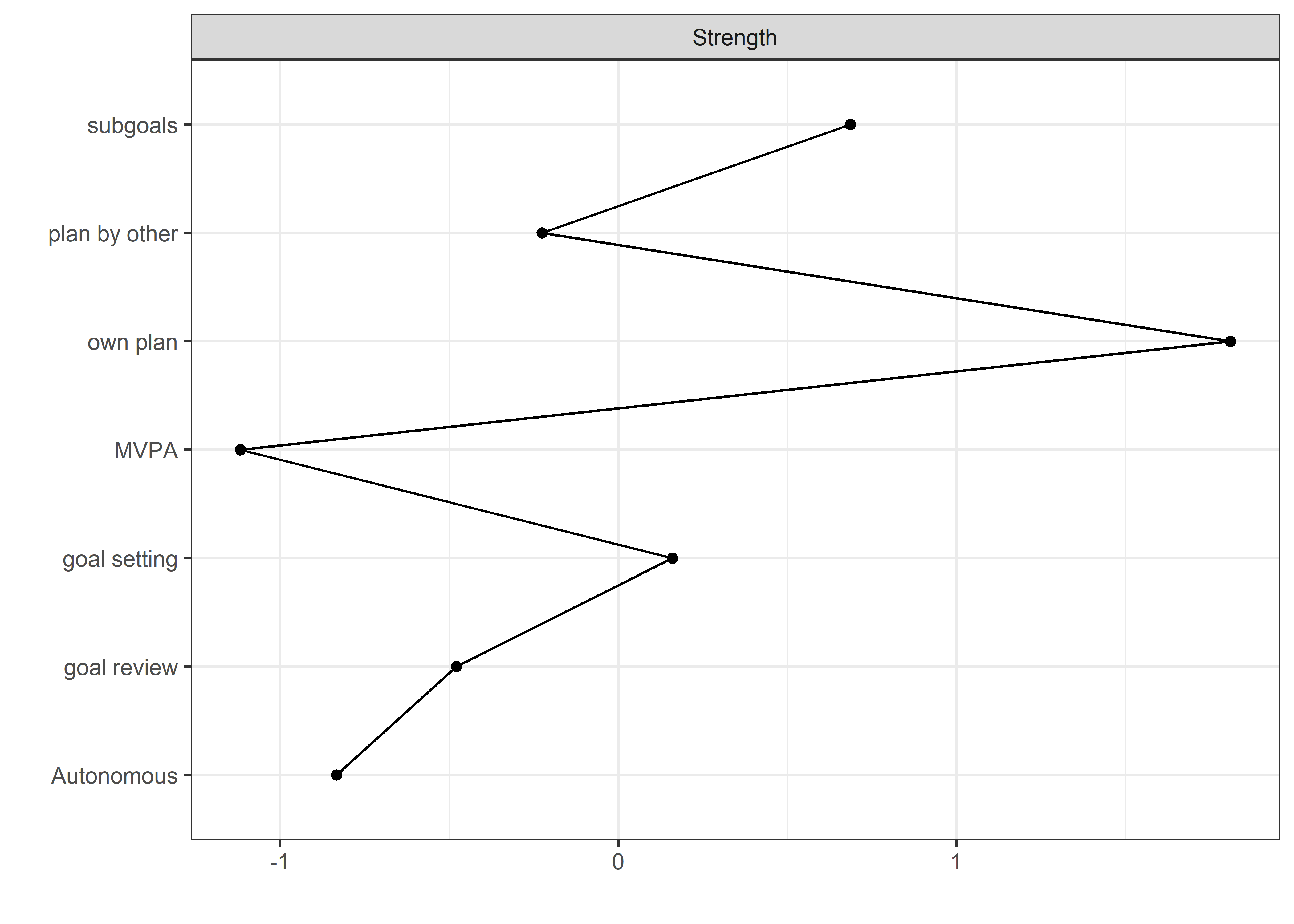
qgraph::centrality(graph_Ising)$InDegree
##          MVPA    Autonomous   goal review      own plan plan by other
##      2.738643      3.198366      3.771397      7.473934      4.181088
##  goal setting      subgoals
##      4.805290      5.656572
scale(qgraph::centrality(graph_Ising)$InDegree)
##                     [,1]
## MVPA          -1.1179740
## Autonomous    -0.8336781
## goal review   -0.4793110
## own plan       1.8103664
## plan by other -0.2259548
## goal setting   0.1600562
## subgoals       0.6864954
## attr(,"scaled:center")
## [1] 4.54647
## attr(,"scaled:scale")
## [1] 1.617056
qgraph::centrality(graph_Ising)$Closeness
##          MVPA    Autonomous   goal review      own plan plan by other
##    0.08689381    0.08758533    0.09784630    0.15833382    0.12275906
##  goal setting      subgoals
##    0.10532717    0.13454803
qgraph::centrality(graph_Ising)$Betweenness
##          MVPA    Autonomous   goal review      own plan plan by other
##             0             0             0            16             4
##  goal setting      subgoals
##             0             2

cor(qgraph::centrality(graph_Ising)$InDegree, qgraph::centrality(graph_Ising)$Betweenness,
    method = "spearman")
## [1] 0.7290021

# bootnet_stability_top5Bcts <- bootnet::bootnet(network_all, stepwise = FALSE, nBoots=1000)
# save(bootnet_stability_top5Bcts, file = "./Rdata_files/bootnet_stability_top5Bcts.Rdata")
load("./Rdata_files/bootnet_stability_top5Bcts.Rdata")

plot(bootnet_stability_top5Bcts, labels = TRUE, order = "sample") 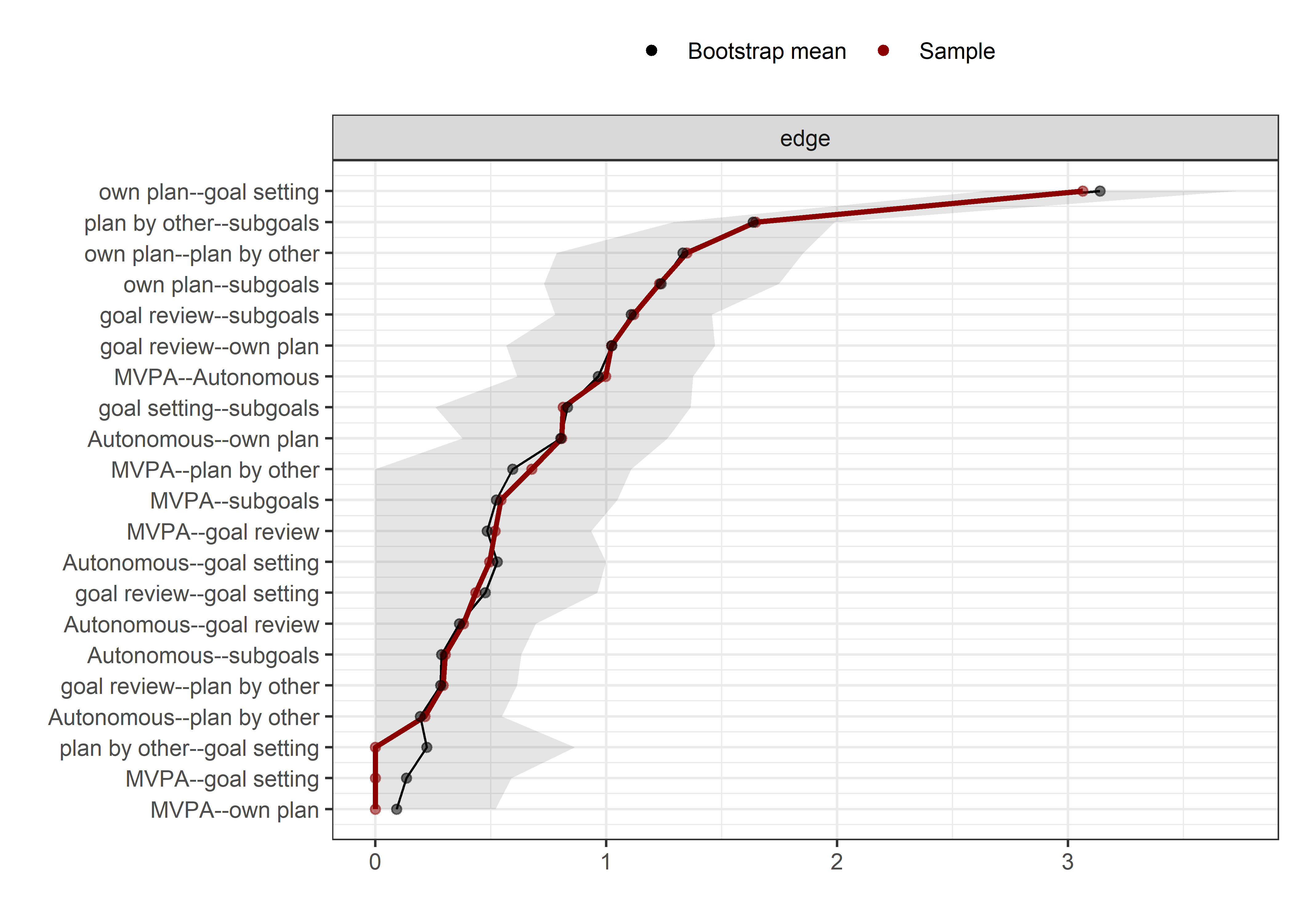
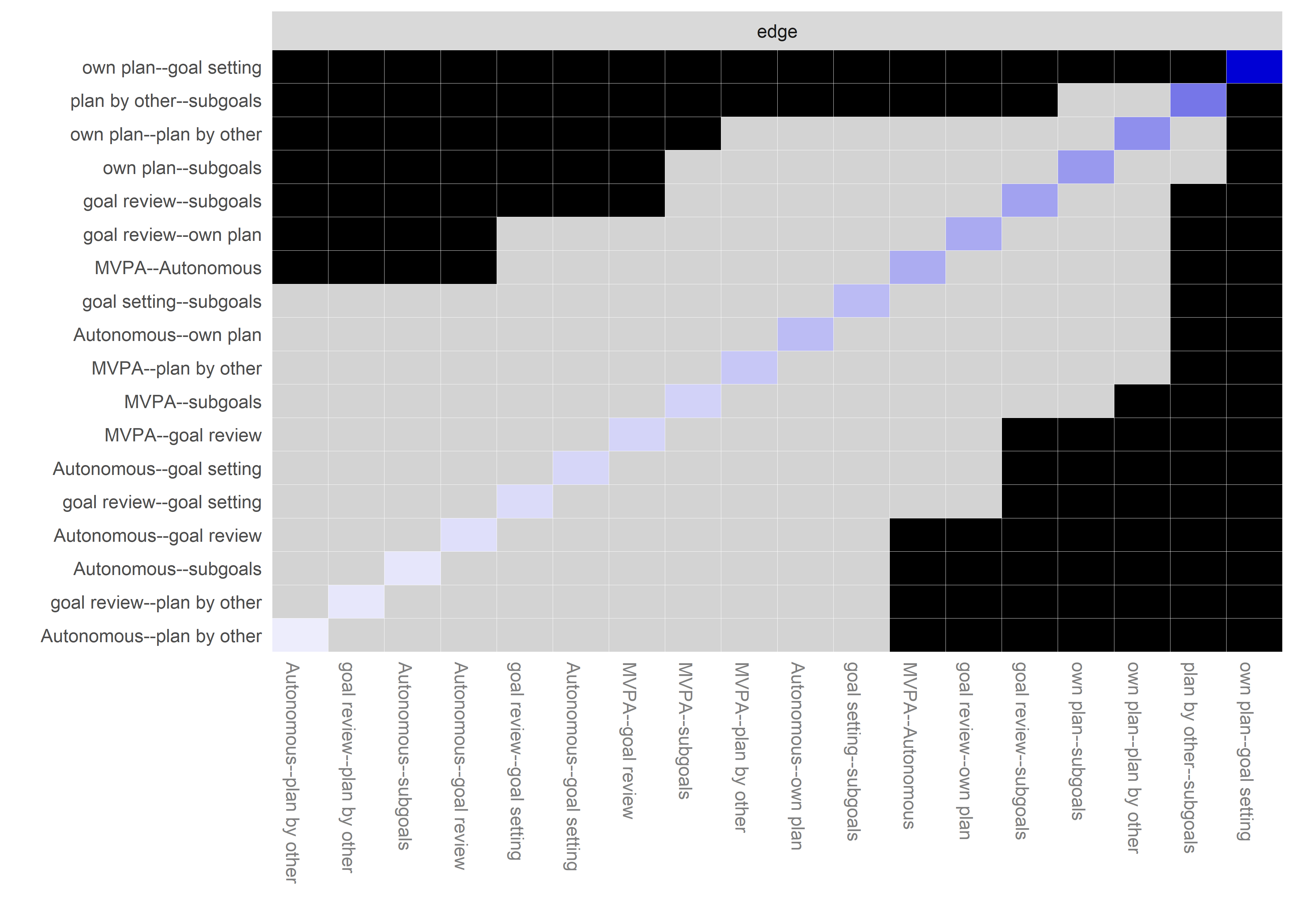
# bootnet_centrality_stability_top5Bcts <- bootnet::bootnet(network_all, stepwise = FALSE, nBoots=1000,nCores=8, type="case")
# save(bootnet_centrality_stability_top5Bcts, file = "./Rdata_files/bootnet_centrality_stability_top5Bcts.Rdata")
# load("./Rdata_files/bootnet_centrality_stability_top5Bcts.Rdata")
#
# plot(bootnet_centrality_stability_top5Bcts)
# plot(bootnet_centrality_stability_top5Bcts, perNode=T, "strength")
#
# bootnet::corStability(bootnet_centrality_stability_top5Bcts)
Heterogeneity check
top5Bcts_tracks_df <- df %>% dplyr::select(
  track,
  PA = padaysLastweek_T1,
  Autonomous = PA_autonomous_T1,
  'trying new PA' = PA_agreementDependentBCT_06_T1,
  'own plan' = PA_agreementDependentBCT_02_T1,
  'plan by other' = PA_agreementDependentBCT_03_T1,
  'goal setting' = PA_agreementDependentBCT_01_T1,
  'subgoals' = PA_agreementDependentBCT_05_T1) %>%
 mutate(
  'PA' = ifelse(`PA` == 0, 0, 1),
  'Autonomous' = ifelse(`Autonomous` < 3, 0, 1),
  'trying new PA' = ifelse(`trying new PA` == 1, 0, 1),
  'own plan' = ifelse(`own plan` == 1, 0, 1),
  'plan by other' = ifelse(`plan by other` == 1, 0, 1),
  'goal setting' = ifelse(`goal setting` == 1, 0, 1),
  'subgoals' = ifelse(`subgoals` == 1, 0, 1))

heterogeneity_Nur <- top5Bcts_tracks_df %>%
  dplyr::filter(track == "Nur") %>%
  dplyr::select(-track) %>%
  na.omit()
NurMeans <- heterogeneity_Nur %>%
  summarise_all(funs(mean(., na.rm = TRUE)))

heterogeneity_HRC <- top5Bcts_tracks_df %>%
  dplyr::filter(track == "HRC") %>%
  dplyr::select(-track) %>%
  na.omit()
HRCMeans <- heterogeneity_HRC %>%
  summarise_all(funs(mean(., na.rm = TRUE)))

heterogeneity_BA <- top5Bcts_tracks_df %>%
  dplyr::filter(track == "BA") %>%
  dplyr::select(-track) %>%
  na.omit()
BAMeans <- heterogeneity_BA %>%
  summarise_all(funs(mean(., na.rm = TRUE)))

heterogeneity_IT <- top5Bcts_tracks_df %>%
  dplyr::filter(track == "IT") %>%
  dplyr::select(-track) %>%
  na.omit()
ITMeans <- heterogeneity_IT %>%
  summarise_all(funs(mean(., na.rm = TRUE)))

network_Nur <- bootnet::estimateNetwork(heterogeneity_Nur, default="IsingFit")
##
  |
  |                                                                 |   0%
  |
  |=========                                                        |  14%
  |
  |===================                                              |  29%
  |
  |============================                                     |  43%
  |
  |=====================================                            |  57%
  |
  |==============================================                   |  71%
  |
  |========================================================         |  86%
  |
  |=================================================================| 100%
network_HRC <- bootnet::estimateNetwork(heterogeneity_HRC, default="IsingFit")
##
  |
  |                                                                 |   0%
  |
  |=========                                                        |  14%
  |
  |===================                                              |  29%
  |
  |============================                                     |  43%
  |
  |=====================================                            |  57%
  |
  |==============================================                   |  71%
  |
  |========================================================         |  86%
  |
  |=================================================================| 100%
network_BA <- bootnet::estimateNetwork(heterogeneity_BA, default="IsingFit")
##
  |
  |                                                                 |   0%
  |
  |=========                                                        |  14%
  |
  |===================                                              |  29%
  |
  |============================                                     |  43%
  |
  |=====================================                            |  57%
  |
  |==============================================                   |  71%
  |
  |========================================================         |  86%
  |
  |=================================================================| 100%
network_IT <- bootnet::estimateNetwork(heterogeneity_IT, default="IsingFit")
##
  |
  |                                                                 |   0%
  |
  |=========                                                        |  14%
  |
  |===================                                              |  29%
  |
  |============================                                     |  43%
  |
  |=====================================                            |  57%
  |
  |==============================================                   |  71%
  |
  |========================================================         |  86%
  |
  |=================================================================| 100%

graph_Nur <- plot(network_Nur, layout="spring", cut=0, label.scale = FALSE,
                  pie = NurMeans, pieBorder = 1, title = "Practical nurse")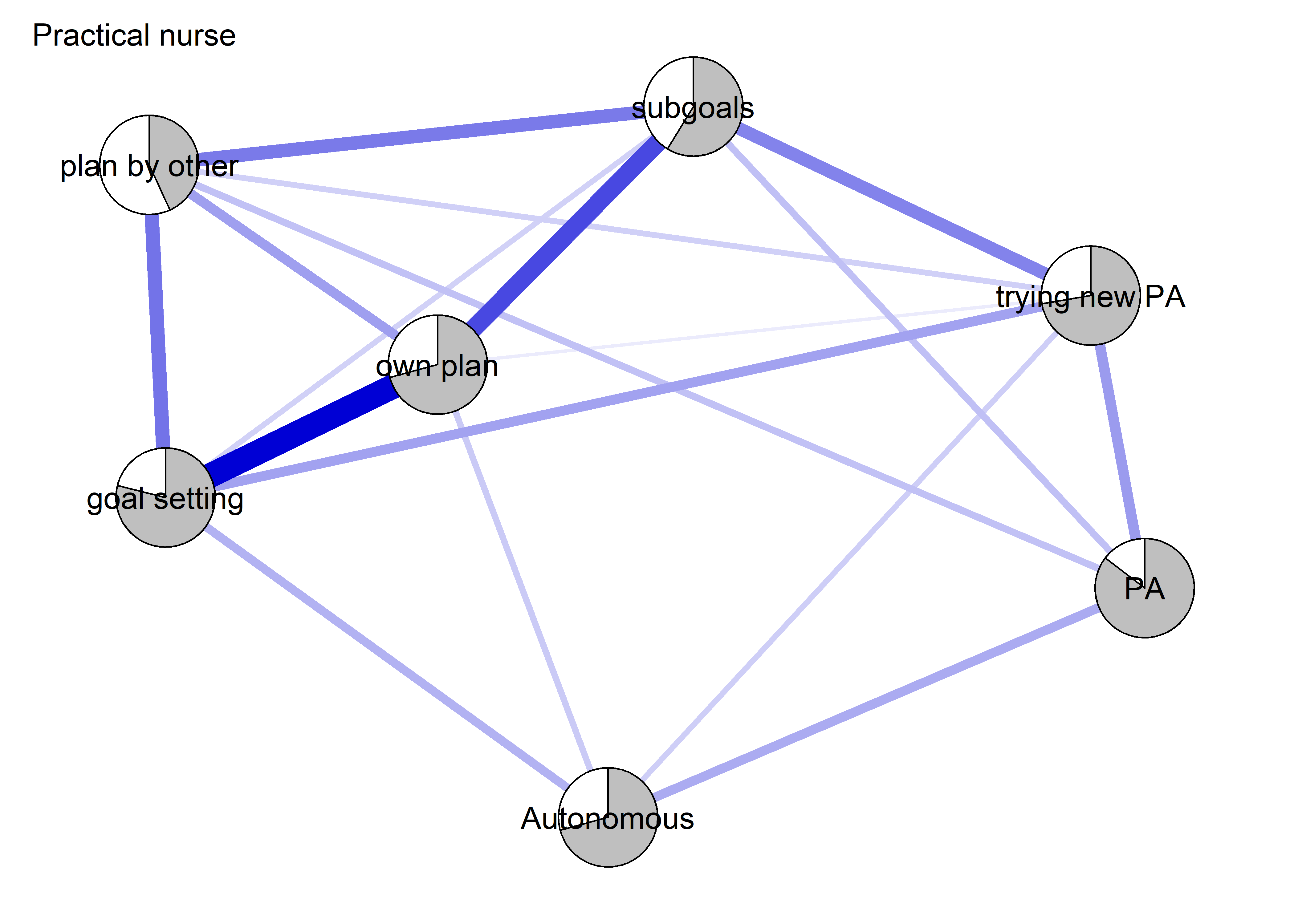
graph_HRC <- plot(network_HRC, layout="spring", cut=0, label.scale = FALSE,
                  pie = HRCMeans, pieBorder = 1, title = "HRC")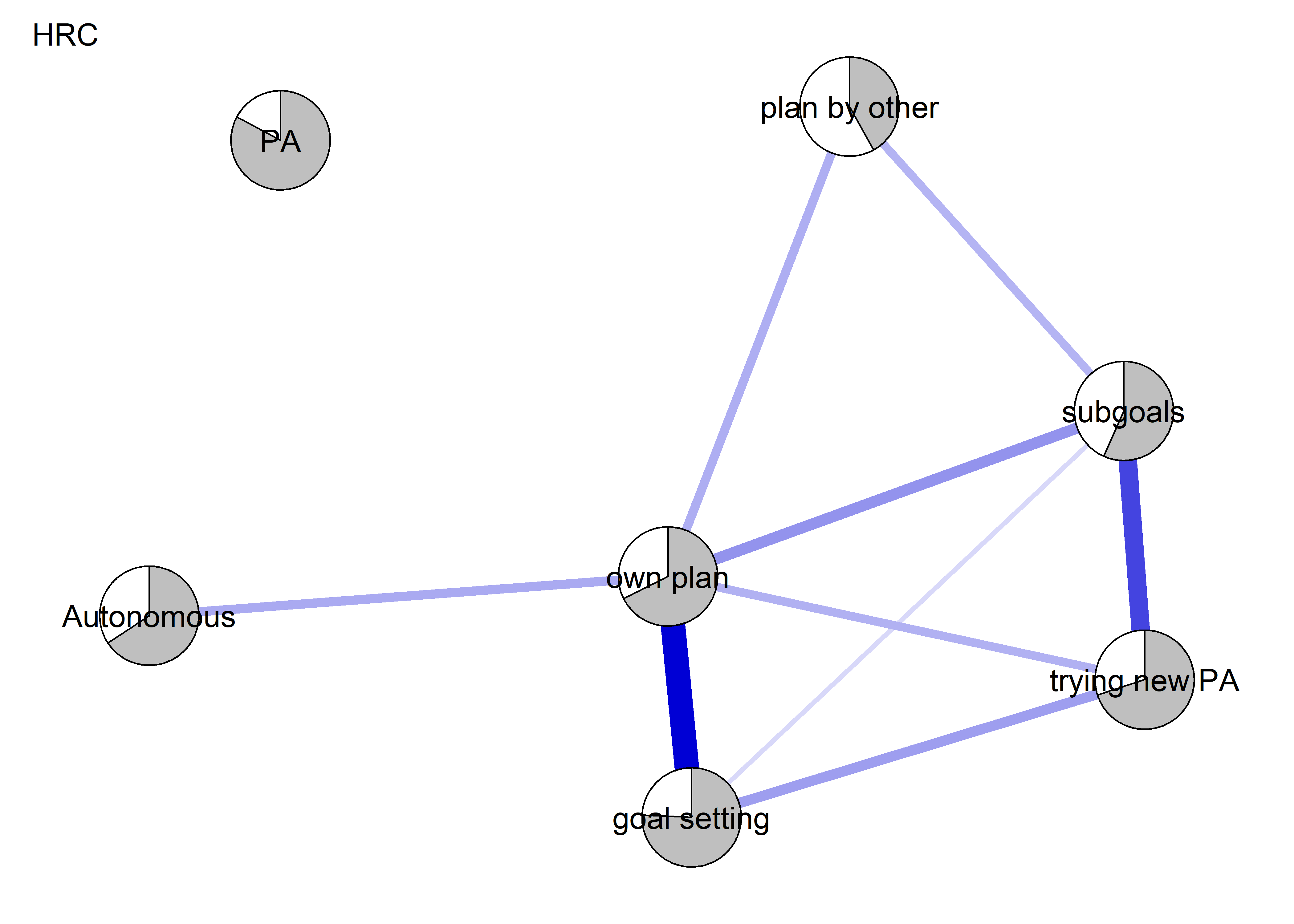
graph_BA <- plot(network_BA, layout="spring", cut=0, label.scale = FALSE,
                  pie = BAMeans, pieBorder = 1, title = "BA")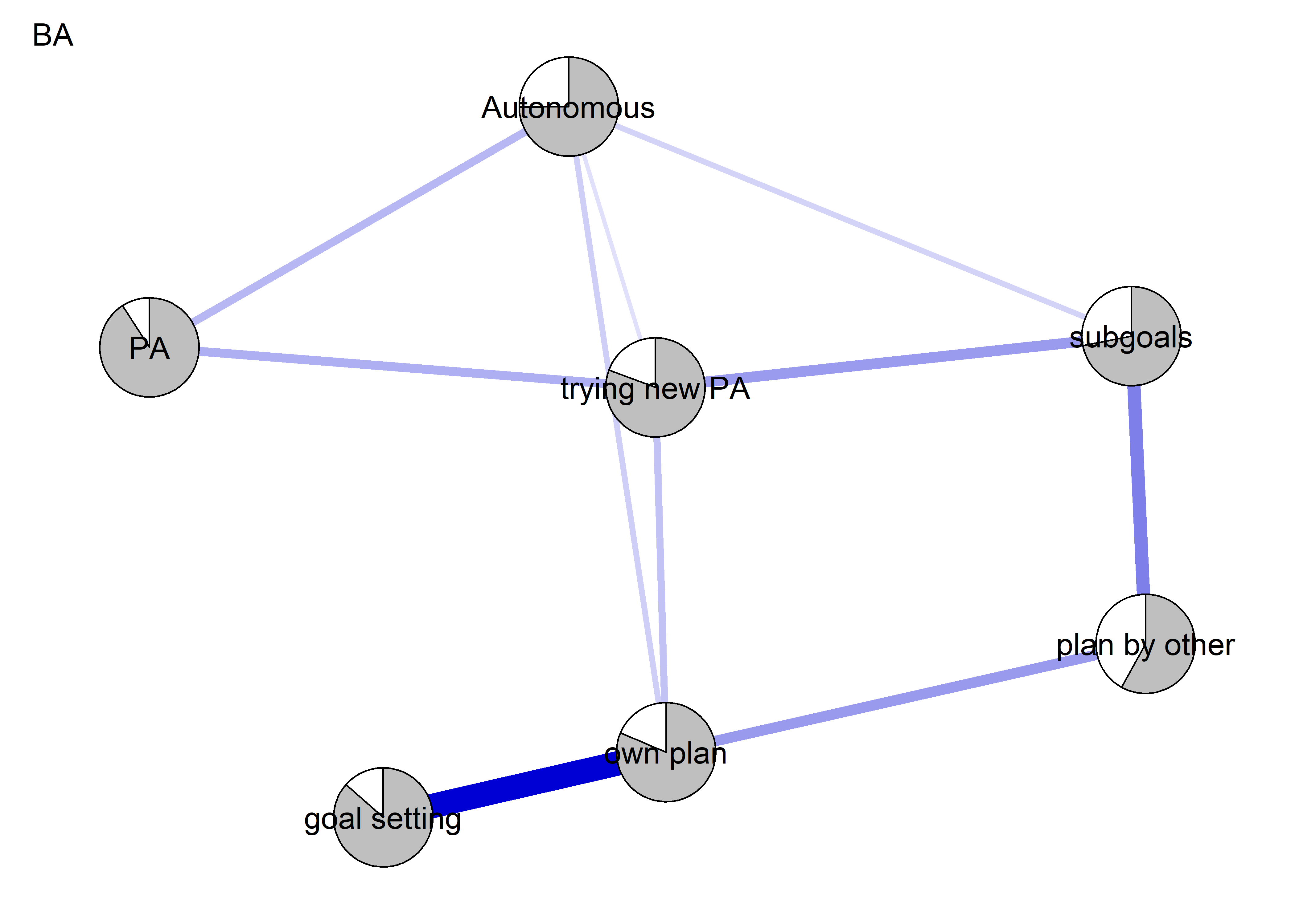
graph_IT <- plot(network_IT, layout="spring", cut=0, label.scale = FALSE,
                  pie = ITMeans, pieBorder = 1, title = "IT")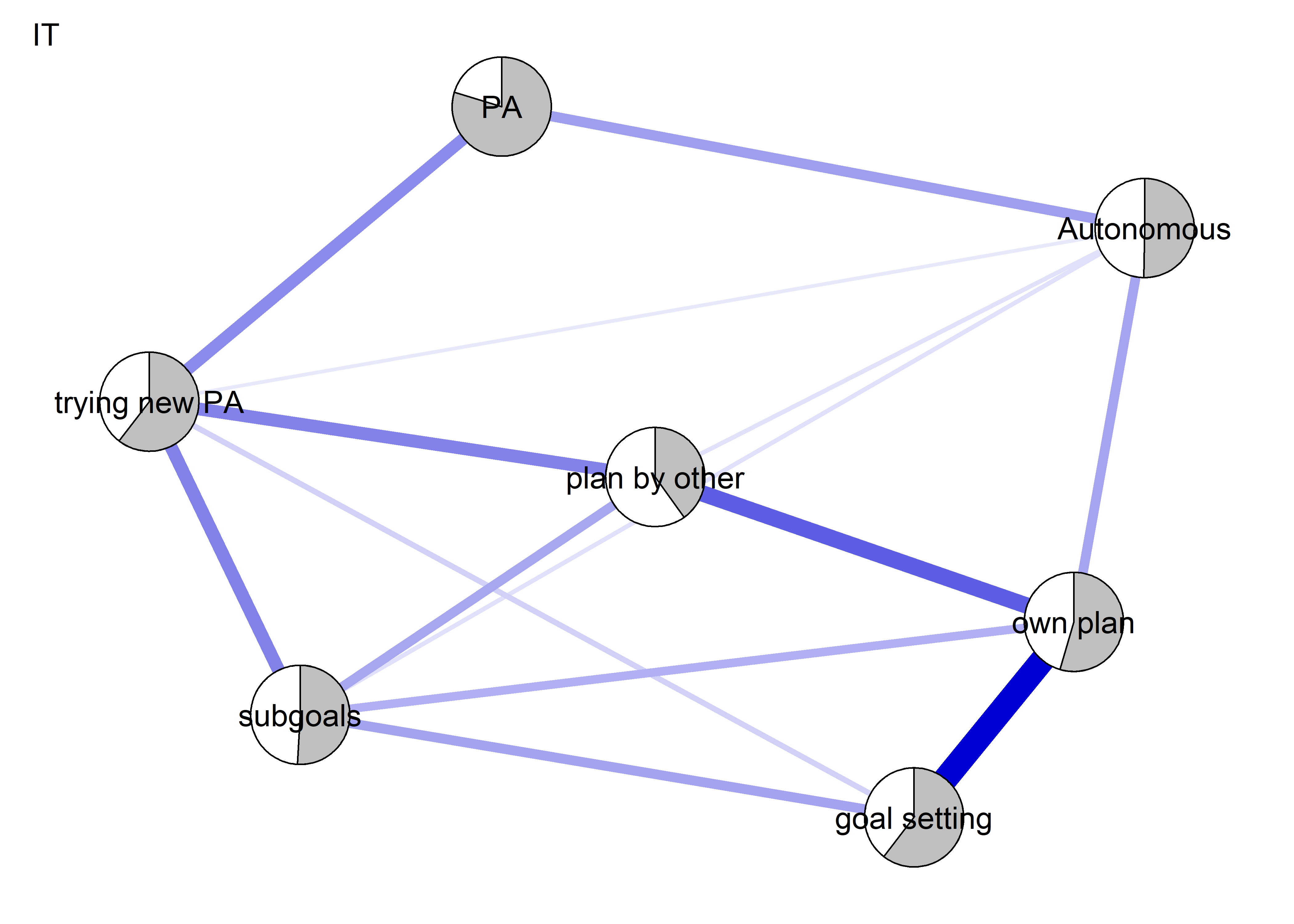
maxedge <- max(c(graph_Nur$graphAttributes$Graph$maximum,
                 graph_HRC$graphAttributes$Graph$maximum,
                 graph_BA$graphAttributes$Graph$maximum,
                 graph_IT$graphAttributes$Graph$maximum))

L <- qgraph::averageLayout(graph_Nur, graph_HRC, graph_BA, graph_IT)

layout(matrix(1:4, nrow = 2, byrow = TRUE))
graph_Nur <- plot(network_Nur, layout=L, cut=0, label.scale = FALSE, title = "Practical nurse",
                  maximum = maxedge, pie = NurMeans, pieBorder = 1)
graph_HRC <- plot(network_HRC, layout=L, cut=0, label.scale = FALSE, title = "HRC",
                  maximum = maxedge, pie = HRCMeans, pieBorder = 1)
graph_BA <- plot(network_BA, layout=L, cut=0, label.scale = FALSE, title = "BA",
                 maximum = maxedge, pie = BAMeans, pieBorder = 1)
graph_IT <- plot(network_IT, layout=L, cut=0, label.scale = FALSE, title = "IT",
                 maximum = maxedge, pie = ITMeans, pieBorder = 1)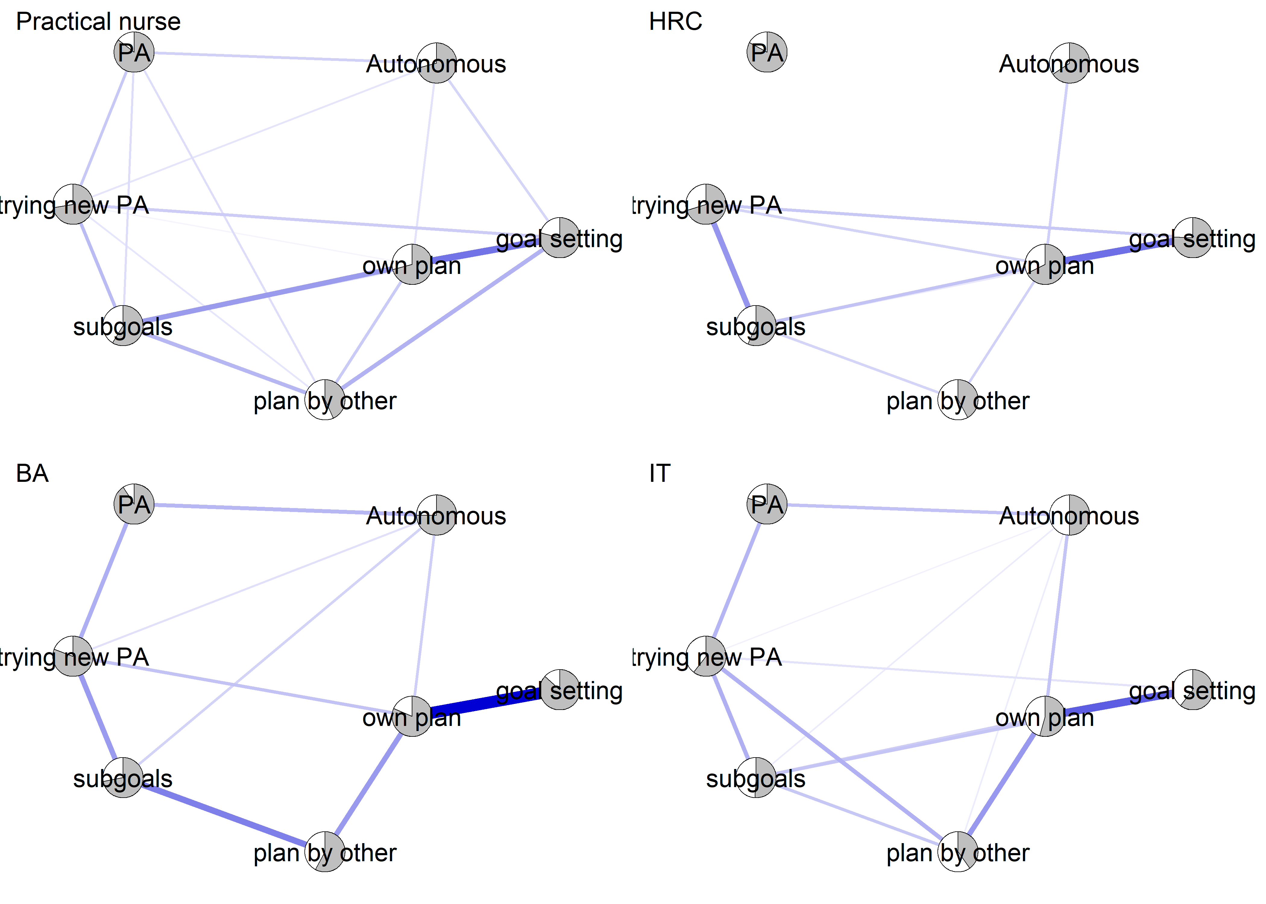
# nct_results_top5Bcts <- NetworkComparisonTest::NCT(heterogeneity_Nur, heterogeneity_IT, it=1000, binary.data=FALSE, paired=FALSE, test.edges=TRUE, edges='all', progressbar=TRUE)
#
# save(nct_results_top5Bcts, file = "./Rdata_files/nct_results_top5Bcts.Rdata")
load("./Rdata_files/nct_results_top5Bcts.Rdata")
Results from the network comparison test between Nur and IT on “top-5” BCTs:
[1] “Similarity”
Correlation between Nur and IT edge strengths: 0.8105599
cat("Correlation between Nur and IT networks:", cor(network_Nur$graph[lower.tri(network_Nur$graph)], network_IT$graph[lower.tri(network_Nur$graph)], method="spearman"))Correlation between Nur and IT networks: 0.4413255
[1] “Difference”
P-value for the test of identical network structure: 0.785
P-value for the test of identical connectivity in networks: 0.217
nct_results_top5Bcts$einv.pvals %>%
papaja::apa_table(caption = "p-values on difference test in edges between Nur and IT")| Var1 | Var2 | p-value | |
|---|---|---|---|
| 8 | PA | Autonomous | 1.00 |
| 15 | PA | trying new PA | 1.00 |
| 16 | Autonomous | trying new PA | 1.00 |
| 22 | PA | own plan | 1.00 |
| 23 | Autonomous | own plan | 1.00 |
| 24 | trying new PA | own plan | 1.00 |
| 29 | PA | plan by other | 1.00 |
| 30 | Autonomous | plan by other | 1.00 |
| 31 | trying new PA | plan by other | 1.00 |
| 32 | own plan | plan by other | 1.00 |
| 36 | PA | goal setting | 1.00 |
| 37 | Autonomous | goal setting | 1.00 |
| 38 | trying new PA | goal setting | 1.00 |
| 39 | own plan | goal setting | 1.00 |
| 40 | plan by other | goal setting | 1.00 |
| 43 | PA | subgoals | 1.00 |
| 44 | Autonomous | subgoals | 1.00 |
| 45 | trying new PA | subgoals | 1.00 |
| 46 | own plan | subgoals | 1.00 |
| 47 | plan by other | subgoals | 1.00 |
| 48 | goal setting | subgoals | 1.00 |
cat("Number of edges, which appear different (p<0.05):", sum(nct_results_top5Bcts$einv.pvals$"p-value" < 0.05))Number of edges, which appear different (p<0.05): 0
PA determinants: unregularised correlations visualised
# Network without motivation variables
data <- df %>% dplyr::select('PA' = mvpaAccelerometer_T1, 'SB' = sitLieAccelerometer_T1,
'fat%' = fatpct_T1,'action planning' = PA_actionplan_T1, 'coping planning' = PA_copingplan_T1, 'frequency-related BCTs' = PA_frequencyDependentBCT_T1, 'agreement-related BCTs' = PA_agreementDependentBCT_T1, 'amotivation' = PA_amotivation_T1, 'autonomous motivation' = PA_autonomous_T1, 'controlled motivation' = PA_controlled_T1, 'descriptive norm' = PA_descriptiveNorm_T1, 'injunctive norm' = PA_injunctiveNorm_T1, 'intention' = PA_intention_T1, 'outcome expectations' = PA_outcomeExpectations_T1, 'self-efficacy / perceivedBehaviouralControl' = PA_selfEfficacyperceivedBehaviouralControl_T1, 'perceived opportunities' = PA_opportunities_T1) %>%
  mutate_all(as.numeric)

names <- df %>% dplyr::select('PA' = mvpaAccelerometer_T1, 'SB' = sitLieAccelerometer_T1,
'fat%' = fatpct_T1,'action planning' = PA_actionplan_T1, 'coping planning' = PA_copingplan_T1, 'frequency-related BCTs' = PA_frequencyDependentBCT_T1, 'agreement-related BCTs' = PA_agreementDependentBCT_T1, 'amotivation' = PA_amotivation_T1, 'autonomous motivation' = PA_autonomous_T1, 'controlled motivation' = PA_controlled_T1, 'descriptive norm' = PA_descriptiveNorm_T1, 'injunctive norm' = PA_injunctiveNorm_T1, 'intention' = PA_intention_T1, 'outcome expectations' = PA_outcomeExpectations_T1, 'self-efficacy / perceivedBehaviouralControl' = PA_selfEfficacyperceivedBehaviouralControl_T1, 'perceived opportunities' = PA_opportunities_T1) %>% names

# Spinglass algorithm detects communities. Tutorial here: http://psych-networks.com/r-tutorial-identify-communities-items-networks/

cormatrix <- qgraph::cor_auto(data)

piefill <- data %>%
  summarise_all(funs(mean(., na.rm = TRUE))) %>%
  mutate_at(vars(PA, SB),
            funs(. / (24*60))) %>% # proportion of day used doing the behaviour
  mutate_at(vars(`action planning`, `coping planning`),
            funs(. / 4)) %>%
  mutate_at(vars(6:ncol(data)),
            funs(. / 7)) %>%
  mutate_at(vars(`fat%`),
            funs(. / 100))

nodeColors <- c(rep(viridis::viridis(7, begin = 0.3, end = 1)[1], 2), # PA, SB
                rep(viridis::viridis(7, begin = 0.3, end = 1)[2], 1), # fat
                rep(viridis::viridis(7, begin = 0.3, end = 1)[3], 2), # Action, coping planning
                rep(viridis::viridis(7, begin = 0.3, end = 1)[4], 2), # 2x bcts
                rep(viridis::viridis(7, begin = 0.3, end = 1)[5], 3), # Motivations
                rep(viridis::viridis(7, begin = 0.3, end = 1)[6], 2), # norms
                rep(viridis::viridis(7, begin = 0.3, end = 1)[7], 1), # intention
                rep(viridis::viridis(7, begin = 0.3, end = 1)[6], 3)) # OE, SE/perceivedBehaviouralControl, Opportunities


qgraph::qgraph(qgraph::cor_auto(data), layout = "spring", labels = TRUE,
       # groups = group.spinglass,
     color=nodeColors,
     label.cex = 0.75,
     label.scale = TRUE,
     pie = piefill,
     color = "skyblue",
     nodeNames = names,
     pieBorder = 1,
     legend.cex = 0.4,
     theme = "colorblind",
     edge.labels = TRUE,
     edge.label.cex = 0.75,
     minimum = 0.1,
     title = "Bivariate correlations of PA determinants (<0.1 not shown)")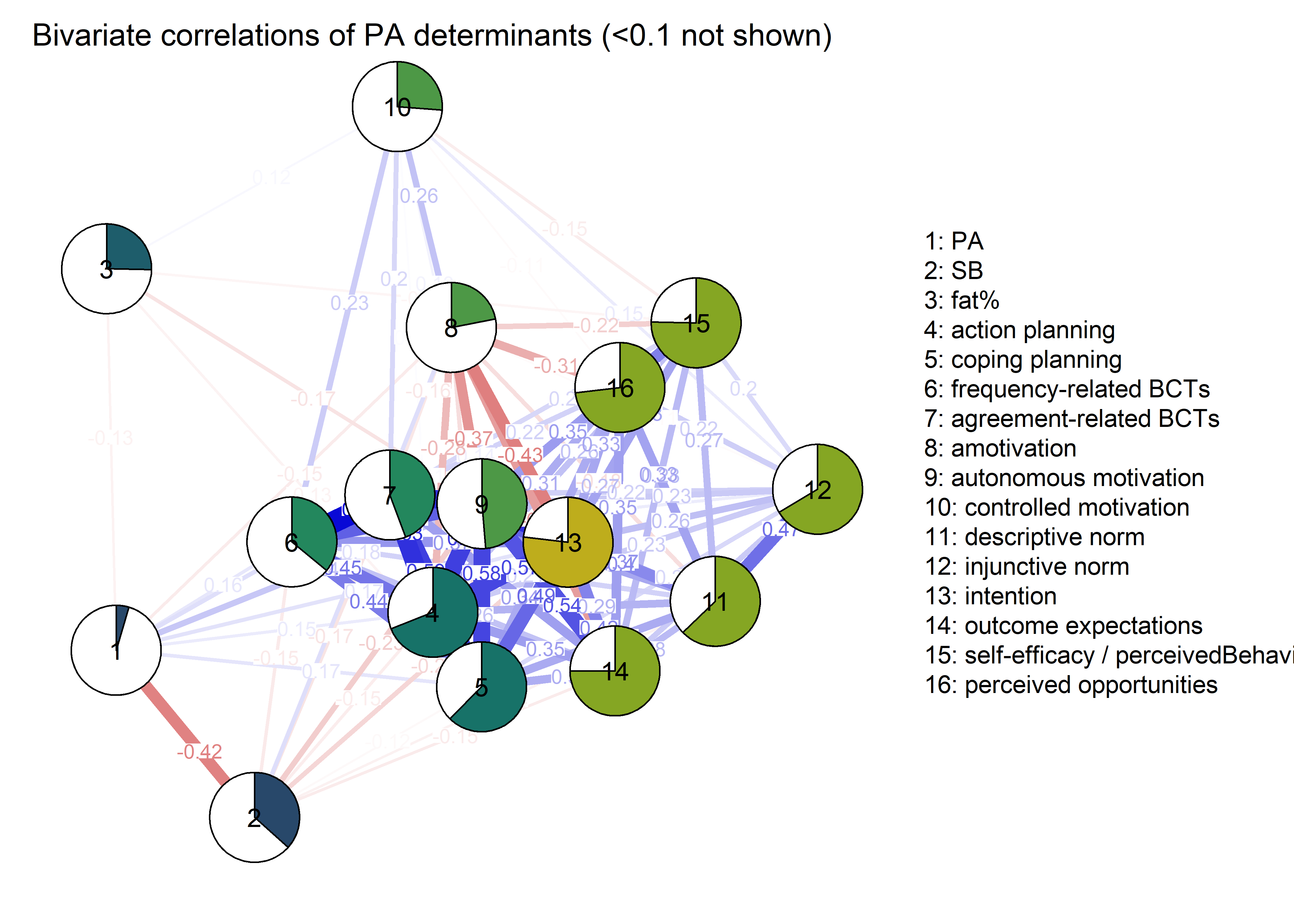
Symptom network: all
sympdf <- df %>% dplyr::select(id,
  intervention,
  group,
  school,
  girl,
  "Neck and shoulder pain" = symptom_neckShoulderPain_T1,
  "Lower back pain" = symptom_lowerBackPain_T1,
  "Stomach ache" = symptom_stomachAche_T1,
  "Tension or nervousness" = symptom_tensionNervousness_T1,
  "Irritability or anger bursts" = symptom_irritabilityAngerbursts_T1,
  "Difficulty with sleep" = symptom_sleepDifficulty_T1,
  "Headache" = symptom_headAche_T1,
  "Tiredness or faintness" = symptom_tirednessFaintness_T1,
  "Fat pct" = fatpct_T1,
  "PA" = mvpaAccelerometer_T1,
  "SB" = sitLieAccelerometer_T1
) %>%
  mutate(
    'Neck and shoulder pain' = ifelse(`Neck and shoulder pain` == 1, 0, 1),
    'Lower back pain' = ifelse(`Lower back pain` == 1, 0, 1),
    'Stomach ache' = ifelse(`Stomach ache` == 1, 0, 1),
    'Tension or nervousness' = ifelse(`Tension or nervousness` == 1, 0, 1),
    'Irritability or anger bursts' = ifelse(`Irritability or anger bursts` == 1, 0, 1),
    'Difficulty with sleep' = ifelse(`Difficulty with sleep` == 1, 0, 1),
    'Headache' = ifelse(`Headache` == 1, 0, 1),
    'Tiredness or faintness' = ifelse(`Tiredness or faintness` == 1, 0, 1),
    'Fat pct' = `Fat pct` / 100) %>%
  data.frame

S.all <- sympdf %>% dplyr::select(6:ncol(sympdf)) %>% na.omit(.)

nwAll <- bootnet::estimateNetwork(S.all, default="mgm")

allmeans <- sympdf %>%
  summarise_at(vars(6:16),
  funs(mean(., na.rm = TRUE))) %>%
  mutate_at(vars(PA, SB),
            funs(. / (24*60)))  # proportion of day used doing the behaviour


plot(nwAll, label.scale = FALSE, title = "All", label.cex = 0.75,
     pie = allmeans,
     color = "skyblue",
     pieBorder = 1)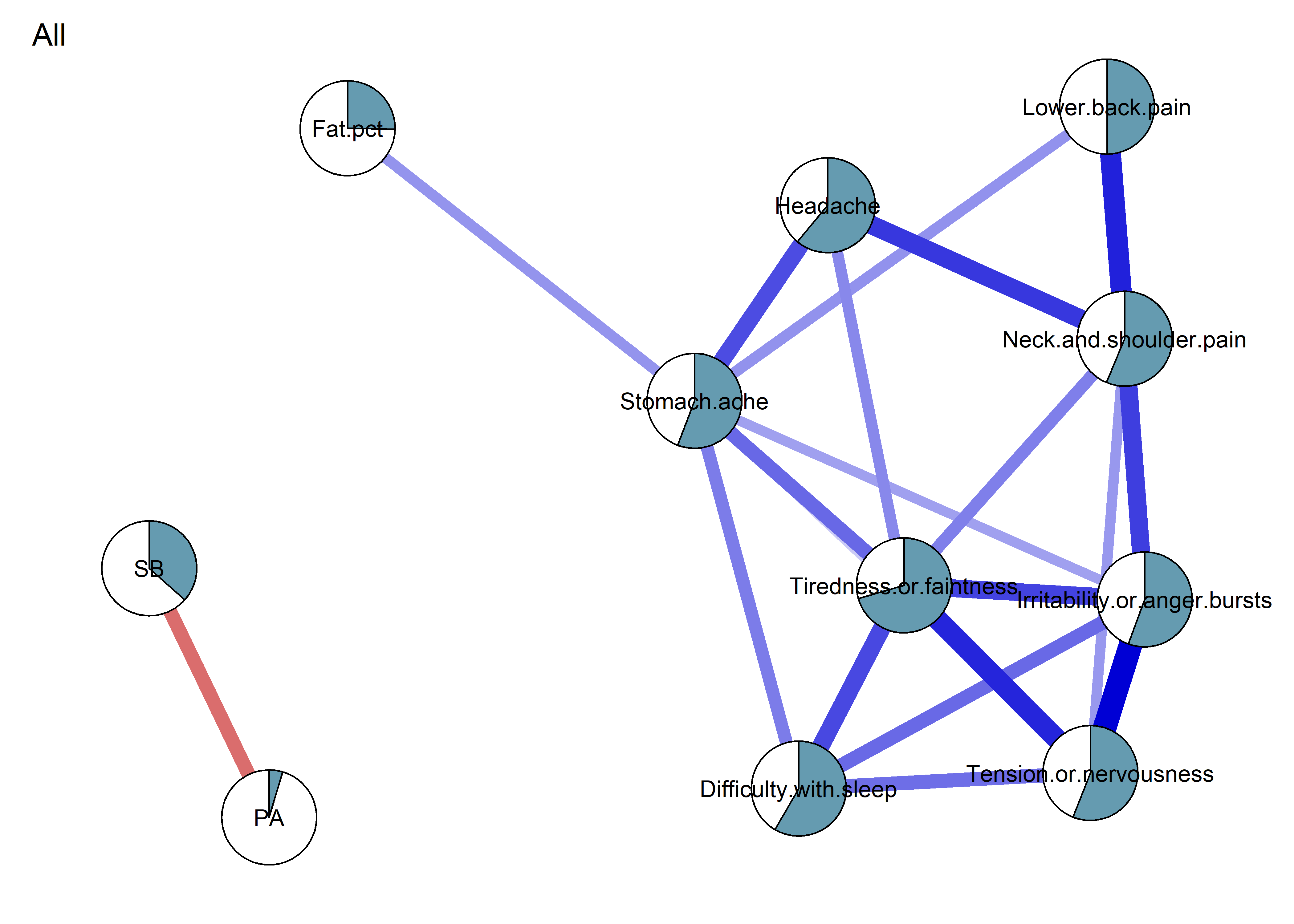
Symptom network: boys and girls
sympdf <- df %>% dplyr::select(id,
  intervention,
  group,
  school,
  girl,
  "Neck and shoulder pain" = symptom_neckShoulderPain_T1,
  "Lower back pain" = symptom_lowerBackPain_T1,
  "Stomach ache" = symptom_stomachAche_T1,
  "Tension or nervousness" = symptom_tensionNervousness_T1,
  "Irritability or anger bursts" = symptom_irritabilityAngerbursts_T1,
  "Difficulty with sleep" = symptom_sleepDifficulty_T1,
  "Headache" = symptom_headAche_T1,
  "Tiredness or faintness" = symptom_tirednessFaintness_T1,
  "Fat pct" = fatpct_T1,
  "PA" = mvpaAccelerometer_T1,
  "SB" = sitLieAccelerometer_T1
) %>%
  mutate(
    'Neck and shoulder pain' = ifelse(`Neck and shoulder pain` == 1, 0, 1),
    'Lower back pain' = ifelse(`Lower back pain` == 1, 0, 1),
    'Stomach ache' = ifelse(`Stomach ache` == 1, 0, 1),
    'Tension or nervousness' = ifelse(`Tension or nervousness` == 1, 0, 1),
    'Irritability or anger bursts' = ifelse(`Irritability or anger bursts` == 1, 0, 1),
    'Difficulty with sleep' = ifelse(`Difficulty with sleep` == 1, 0, 1),
    'Headache' = ifelse(`Headache` == 1, 0, 1),
    'Tiredness or faintness' = ifelse(`Tiredness or faintness` == 1, 0, 1),
    'Fat pct' = `Fat pct` / 100)

S.boys <- sympdf %>% filter(girl == "boy") %>% dplyr::select("Neck and shoulder pain":ncol(sympdf)) %>% na.omit(.)
S.girls <- sympdf %>% filter(girl == "girl") %>% dplyr::select("Neck and shoulder pain":ncol(sympdf)) %>% na.omit(.)
nwBoys <- bootnet::estimateNetwork(S.boys, default="mgm")
nwGirls <- bootnet::estimateNetwork(S.girls, default="mgm")

girlmeans <- sympdf %>% group_by(girl) %>%
  summarise_at(vars("Neck and shoulder pain":"SB"),
  funs(mean(., na.rm = TRUE))) %>%
  filter(girl == "girl") %>%
  mutate_at(vars(PA, SB),
            funs(. / (24*60))) %>% # proportion of day used doing the behaviour
  dplyr::select(-(girl))

boymeans <- sympdf %>% group_by(girl) %>%
  summarise_at(vars("Neck and shoulder pain":"SB"),
  funs(mean(., na.rm = TRUE))) %>%
  filter(girl == "boy") %>%
  mutate_at(vars(PA, SB),
            funs(. / (24*60))) %>% # proportion of day used doing the behaviour
  dplyr::select(-(girl))


layout(t(1:2))
plot(nwGirls, label.scale = FALSE, title = "Girls", label.cex = 0.75,
     pie = girlmeans,
     color = "skyblue",
     pieBorder = 1)

plot(nwBoys, label.scale = FALSE, title = "Boys", label.cex = 0.75,
     pie = boymeans,
     color = "skyblue",
     pieBorder = 1)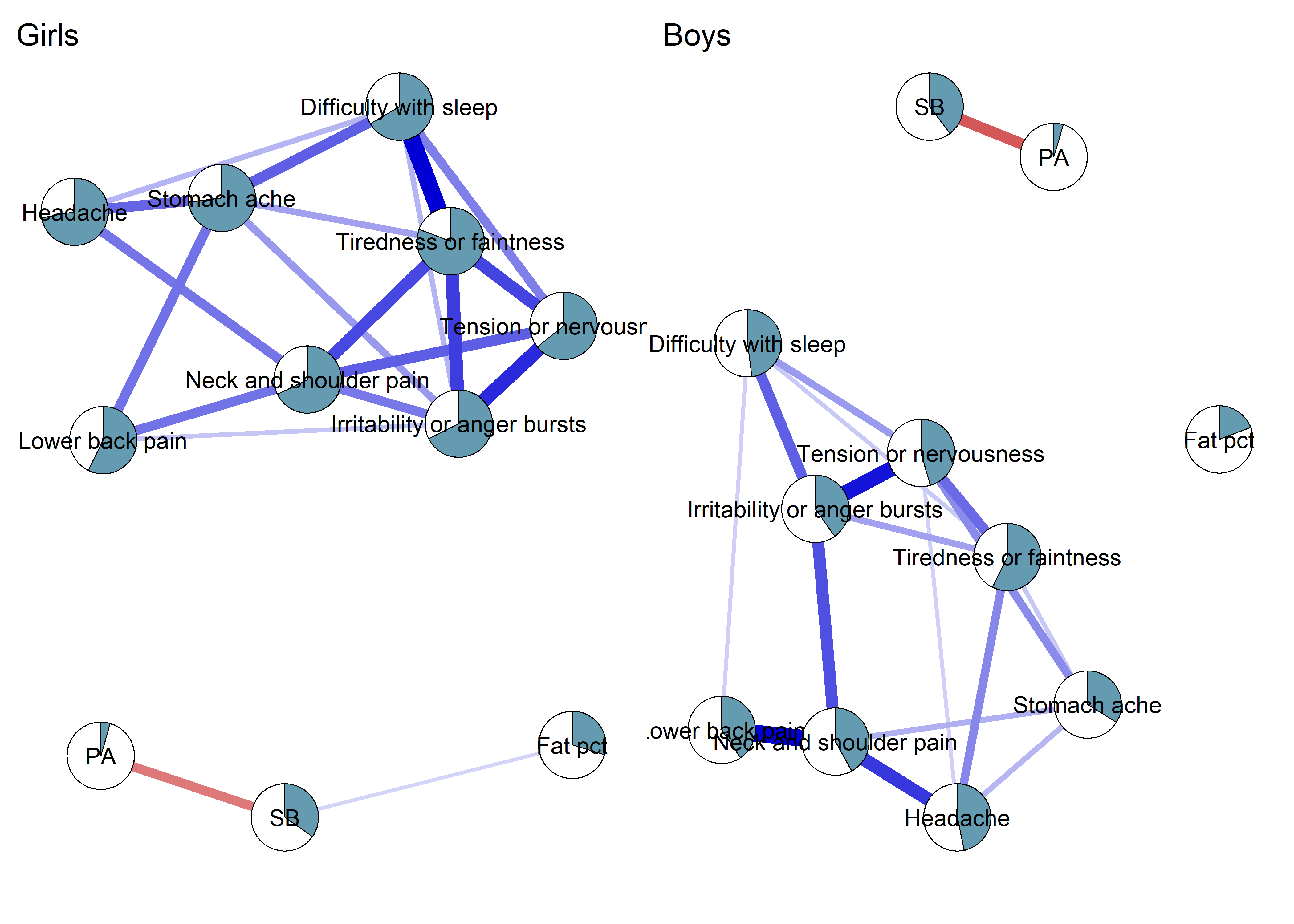
symptom network: educational tracks
PA determinant network
data <- df %>%
  dplyr::select(
    "MVPA accelerometer" = mvpaAccelerometer_T1,
    "planning" = PA_actCop_T1,
    "BCT" = PA_frequencyDependentBCT_T1,
    "amotivation" = PA_amotivation_T1,
    "autonomous" = PA_autonomous_T1,
    "controlled" = PA_controlled_T1,
    "descriptive norm" = PA_descriptiveNorm_T1,
    "fat pct" = fatpct_T1,
    "injunctive norm" = PA_injunctiveNorm_T1,
    "intention" = PA_intention_T1,
    "outcome expectations" = PA_outcomeExpectations_T1,
    "opportunities" = PA_opportunities_T1,
    "self-efficacy perceivedBehaviouralControl" = PA_selfEfficacyperceivedBehaviouralControl_T1) %>%
  mutate_all(funs(as.numeric(.)))

covMatrix <- data %>% cov(use = "pairwise.complete.obs")

# Transform the matrix so, that lower diagonal of the matrix shows partial correlations,
# while the upper one shows bivariate correlations.
matrix_corLower_parcorUpper <- covMatrix %>% ggm::correlations()

# Show the matrix
matrix_corLower_parcorUpper %>% papaja::apa_table(caption = "Correlation matrix of hypothesised determinants. Lower diagonal shows bivariate correlations, upper diagonal shows partial correlations")
## <caption>(\#tab:determinants)</caption>
##
## <caption>*Correlation matrix of hypothesised determinants. Lower diagonal shows bivariate correlations, upper diagonal shows partial correlations*</caption>
##
##
##
##                                             MVPA accelerometer   planning   BCT     amotivation   autonomous   controlled   descriptive norm   fat pct   injunctive norm   intention   outcome expectations   opportunities   self-efficacy perceivedBehaviouralControl
## ------------------------------------------  -------------------  ---------  ------  ------------  -----------  -----------  -----------------  --------  ----------------  ----------  ---------------------  --------------  ------------------------------------------
## MVPA accelerometer                          1.00                 0.01       0.07    -0.09         0.13         -0.02        -0.03              -0.08     0.00              0.01        -0.10                  -0.05           0.06
## planning                                    0.17                 1.00       0.23    0.04          0.27         0.00         0.01               -0.03     0.04              0.25        -0.03                  0.11            0.05
## BCT                                         0.16                 0.47       1.00    0.10          0.26         0.13         0.02               0.06      -0.01             0.06        0.01                   -0.01           -0.11
## amotivation                                 -0.15                -0.25      -0.08   1.00          -0.15        0.29         0.03               -0.07     -0.02             -0.24       -0.14                  -0.12           0.05
## autonomous                                  0.24                 0.62       0.51    -0.37         1.00         0.16         0.08               -0.18     -0.05             0.24        0.32                   0.04            0.08
## controlled                                  -0.02                0.09       0.23    0.26          0.13         1.00         -0.02              0.14      0.16              0.00        0.02                   -0.08           -0.13
## descriptive norm                            0.06                 0.33       0.21    -0.18         0.37         0.04         1.00               -0.05     0.38              0.15        0.00                   0.14            0.05
## fat pct                                     -0.13                -0.12      -0.02   0.03          -0.17        0.12         -0.09              1.00      0.02              0.03        0.11                   0.02            -0.06
## injunctive norm                             0.03                 0.23       0.15    -0.11         0.23         0.15         0.47               0.00      1.00              0.04        0.08                   0.04            0.06
## intention                                   0.17                 0.57       0.37    -0.43         0.63         0.02         0.40               -0.08     0.26              1.00        0.04                   -0.03           0.11
## outcome expectations                        0.05                 0.35       0.26    -0.35         0.54         0.04         0.28               0.01      0.24              0.42        1.00                   0.12            0.06
## opportunities                               0.05                 0.33       0.14    -0.31         0.35         -0.11        0.33               -0.06     0.22              0.33        0.35                   1.00            0.27
## self-efficacy perceivedBehaviouralControl   0.11                 0.28       0.06    -0.22         0.32         -0.15        0.27               -0.12     0.20              0.33        0.28                   0.42            1.00

# Plot the matrix as a correlogram
matrix_corLower_parcorUpper %>% corrgram::corrgram(
  type = "cor",
  lower.panel = corrgram::panel.pie,
  upper.panel = corrgram::panel.pie,
  main = "Bivariate (upper diagonal) and partial (lower diagonal)\ncorrelations of PA determinants")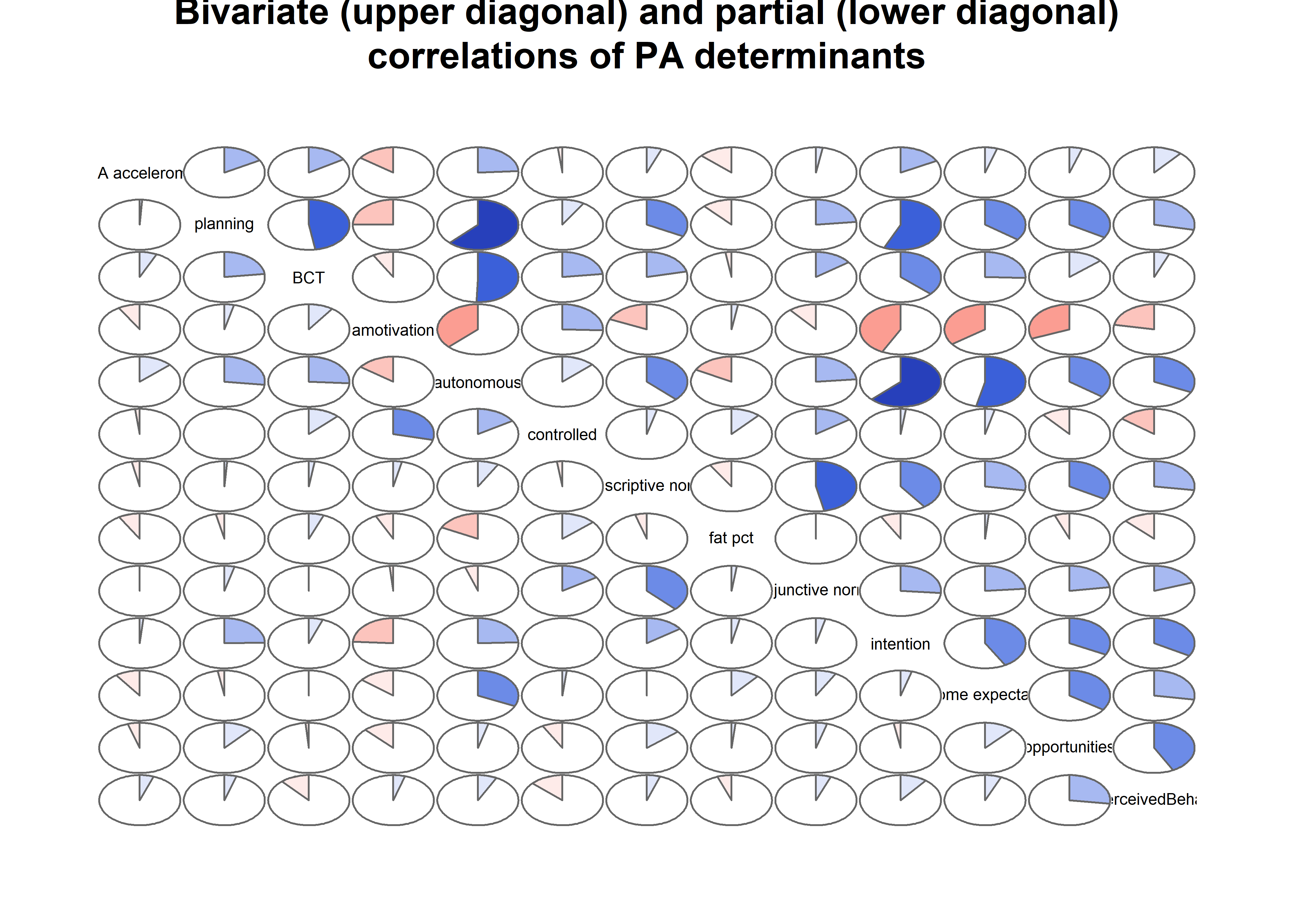
ggm estimation
# Estimate a network

determinants_ggm_network <- bootnet::estimateNetwork(data, default="ggmModSelect")

bootnetgraph <- plot(determinants_ggm_network, edge.labels = TRUE, labels = names(data), label.scale = FALSE,
       title = "ggmModSelect")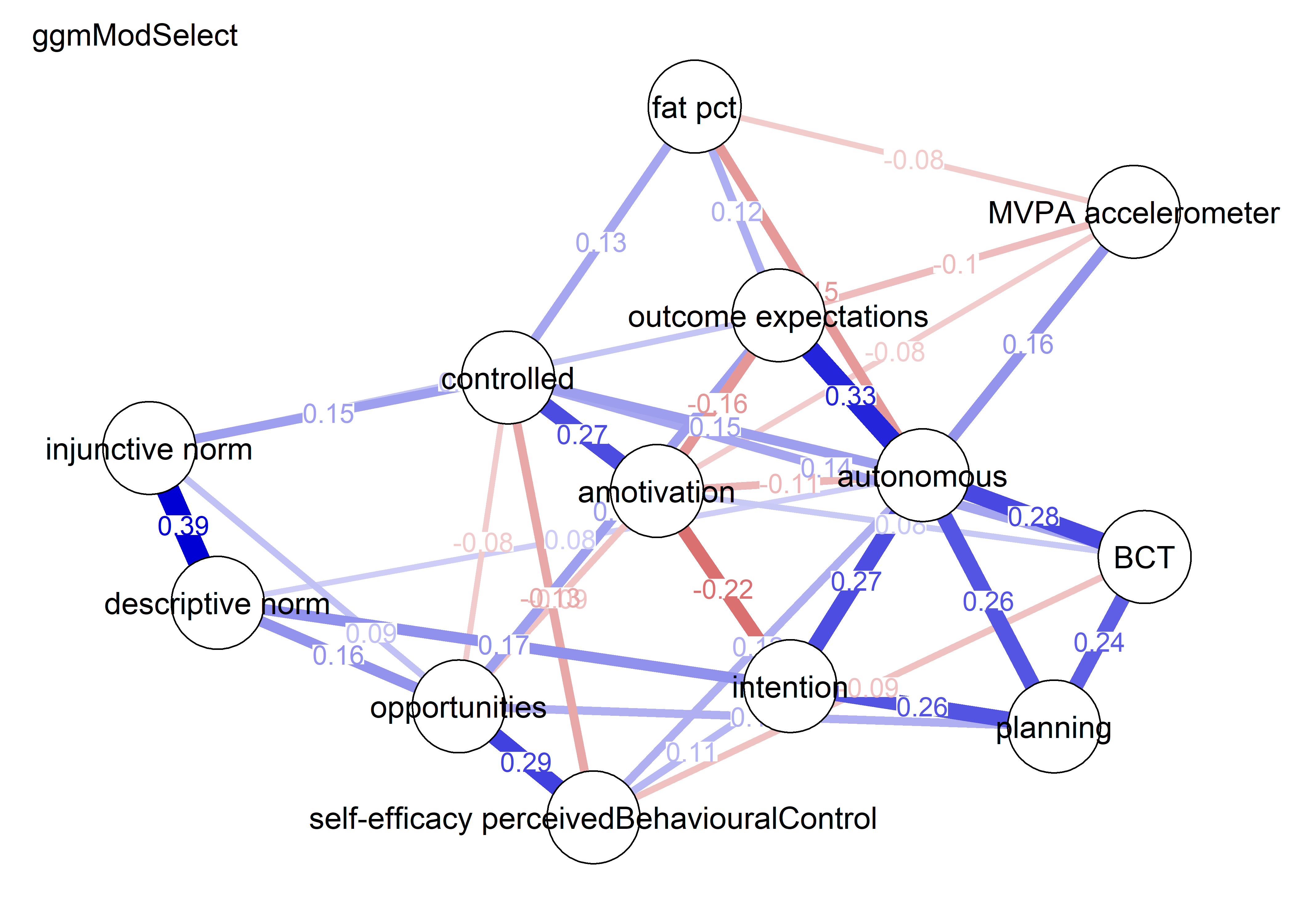
corgraph <- qgraph::qgraph(qgraph::cor_auto(data), graph = "cor",
       labels = names(data),
       label.scale = FALSE,
       edge.labels = TRUE,
       title = "bivariate correlation network")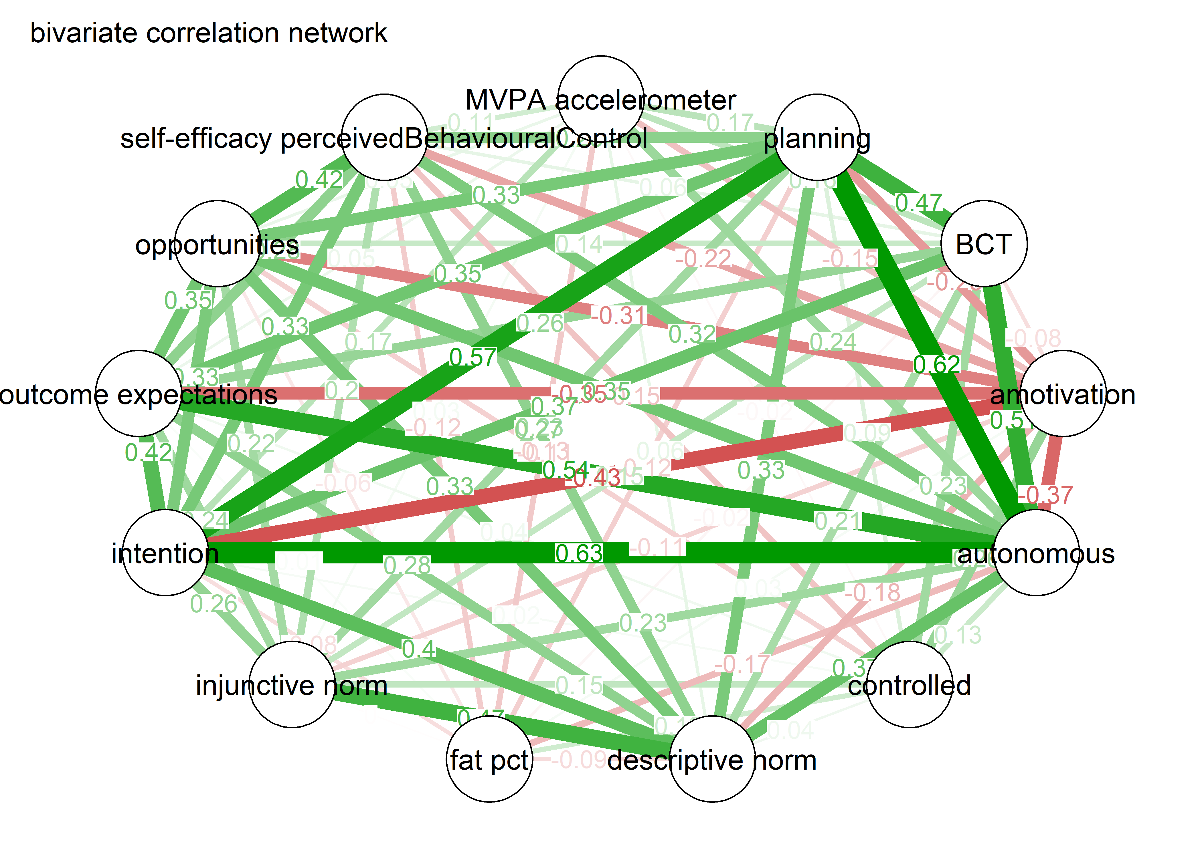
pcorgraph <- qgraph::qgraph(qgraph::cor_auto(data), graph = "pcor",
       labels = names(data),
       label.scale = FALSE,
       edge.labels = TRUE,
       title = "partial correlation network")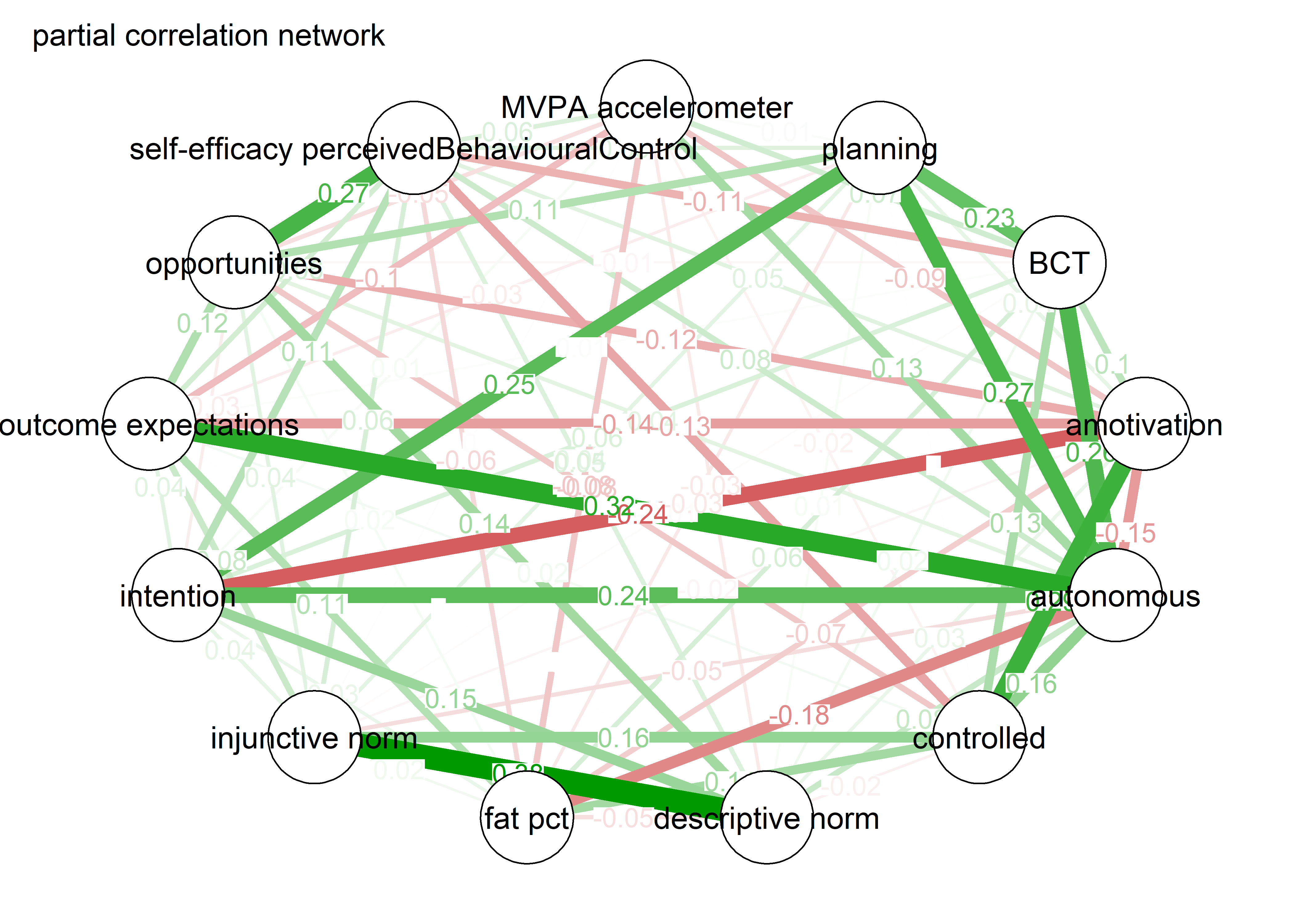
# Average the layout and plot all according to that
avlayout <- qgraph::averageLayout(bootnetgraph, corgraph, pcorgraph)

corgraph <- qgraph::qgraph(qgraph::cor_auto(data), graph = "cor",
       labels = names(data),
       edge.labels = TRUE,
       layout = avlayout,
       title = "bivariate correlation network",
       theme = "colorblind",
       maximum = max(c(bootnetgraph$graph$Graph$maximum,
                     pcorgraph$graph$Graph$maximum,
                     corgraph$graph$Graph$maximum)),
       label.scale = FALSE)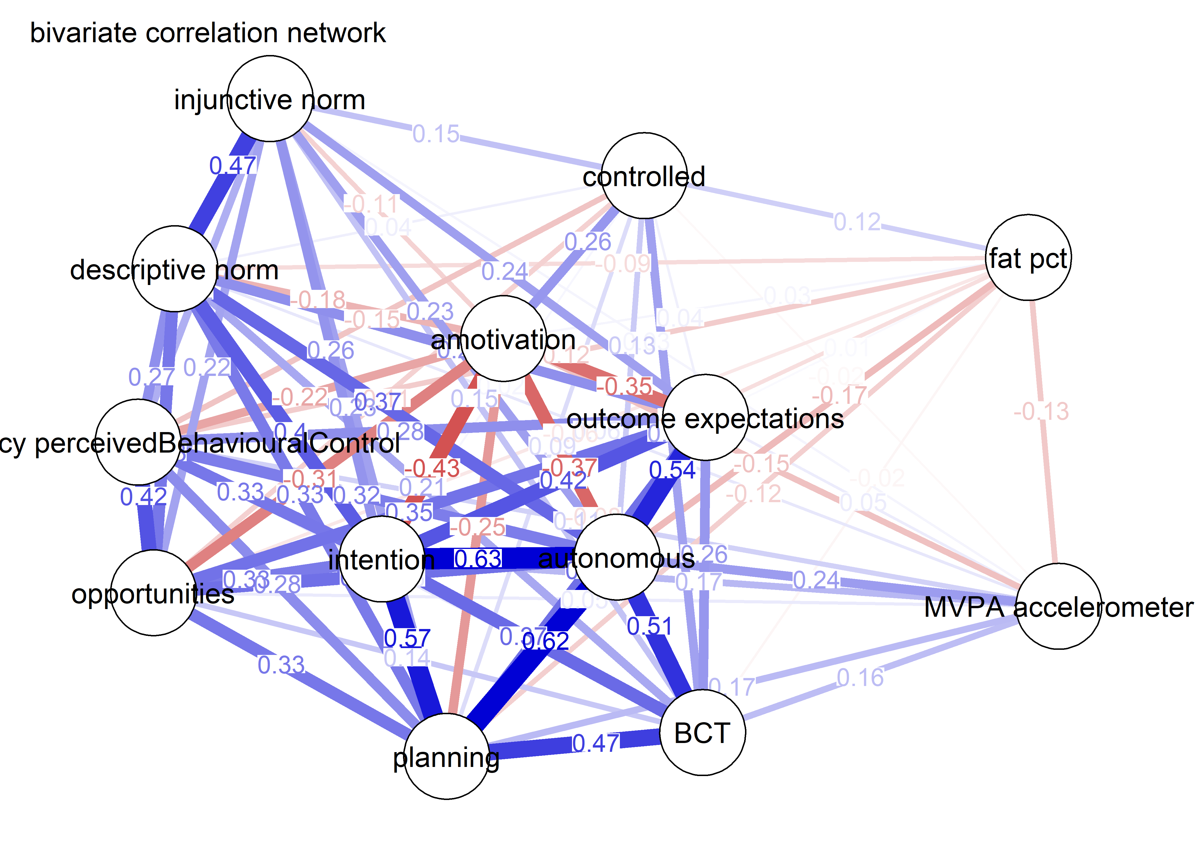
# To help with visual comparison, that last argument takes the maximum edge of the three
# graphs and places that as the benchmark for the thickest line in all plots.

pcorgraph <- qgraph::qgraph(qgraph::cor_auto(data), graph = "pcor",
       labels = names(data),
       edge.labels = TRUE,
       layout = avlayout,
       title = "partial correlation network",
       theme = "colorblind",
       maximum = max(c(bootnetgraph$graph$Graph$maximum,
                     pcorgraph$graph$Graph$maximum,
                     corgraph$graph$Graph$maximum)),
       label.scale = FALSE)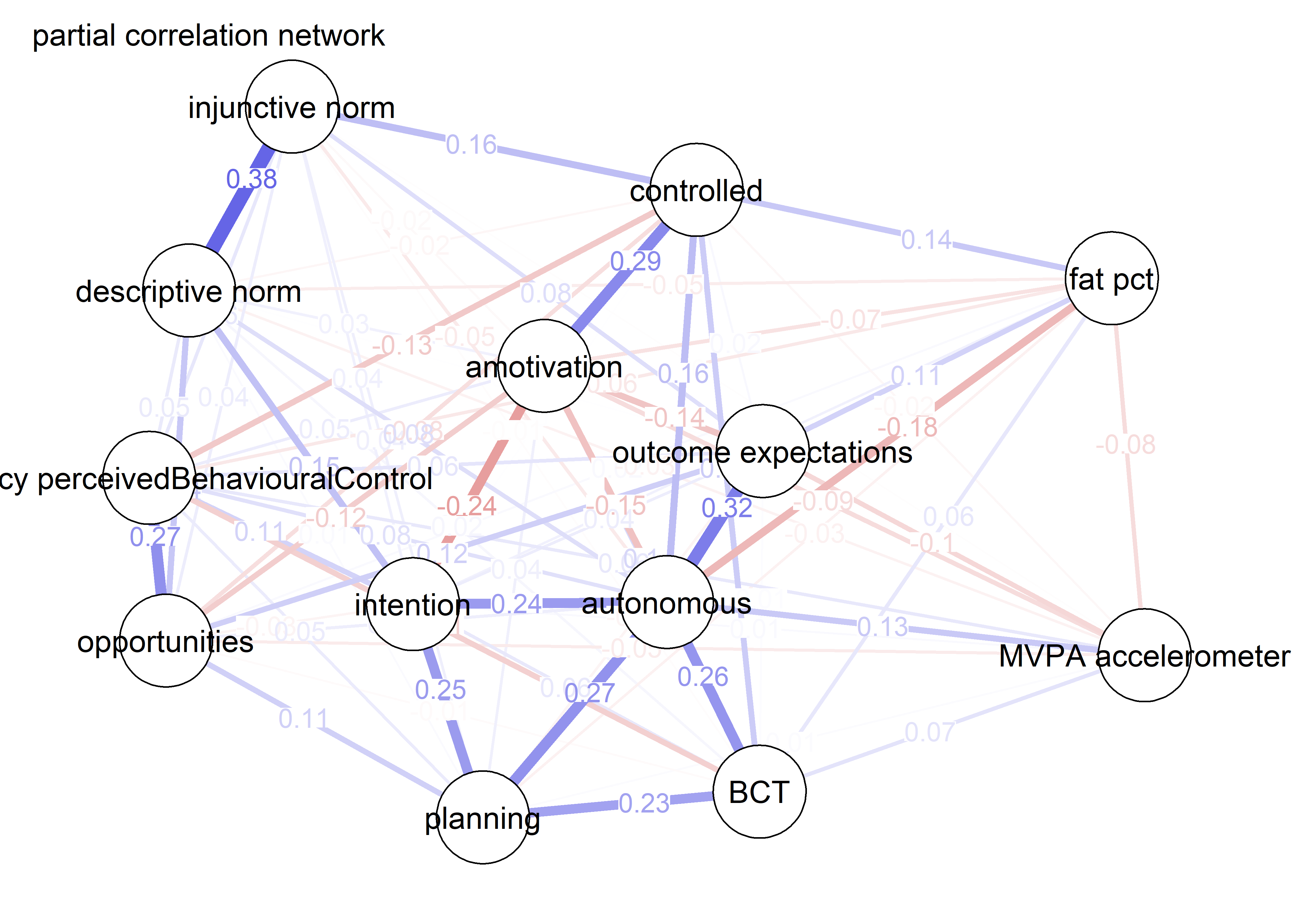
bootnetgraph <- plot(determinants_ggm_network,
                     edge.labels = TRUE,
                     layout = avlayout,
                     title = "ggmModSelect",
       maximum = max(c(bootnetgraph$graph$Graph$maximum,
                     pcorgraph$graph$Graph$maximum,
                     corgraph$graph$Graph$maximum)),
       label.scale = FALSE)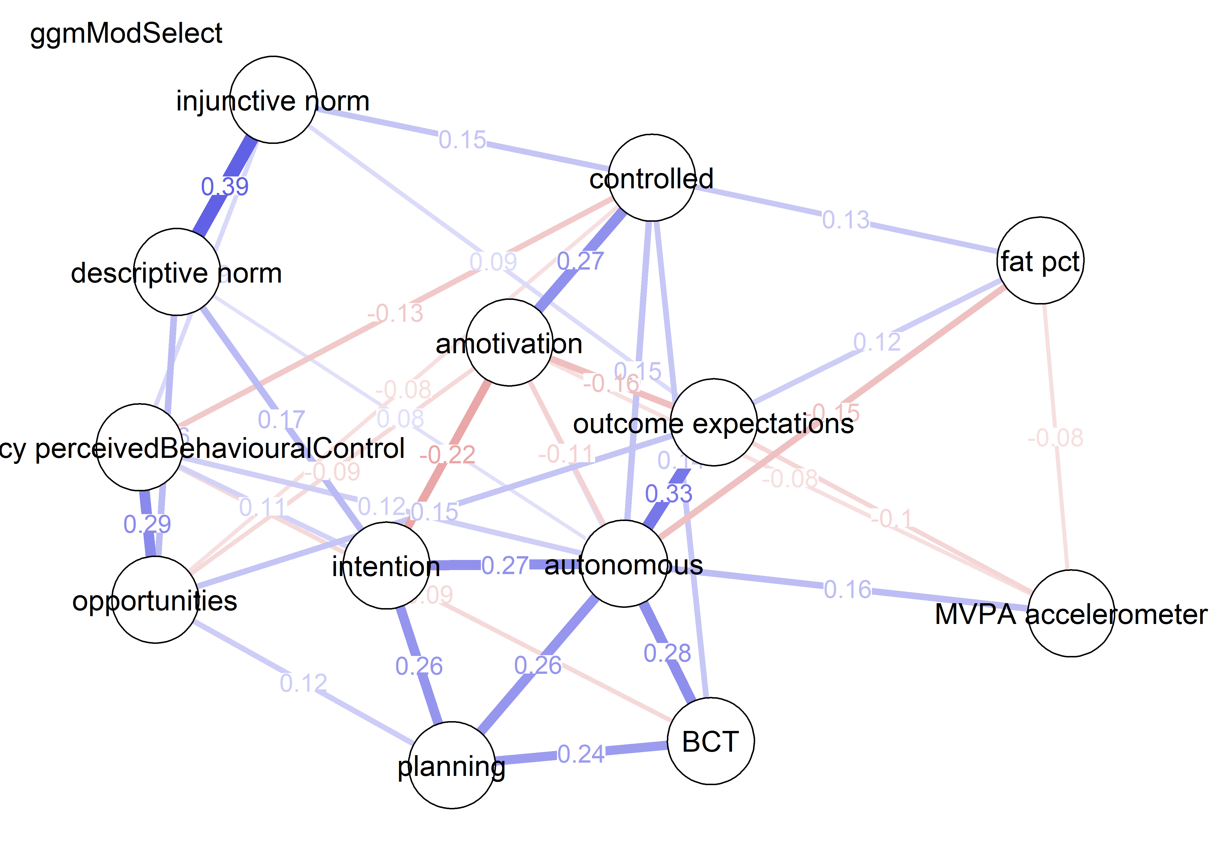
A dressed-up version of the last graph. Pies indicate mean as a proportion of the maximum observed value in that variable in question.
data <- df %>%
  dplyr::select(
    "MVPA accelerometer" = mvpaAccelerometer_T1,
    "planning" = PA_actCop_T1,
    "BCT" = PA_frequencyDependentBCT_T1,
    "amotivation" = PA_amotivation_T1,
    "autonomous" = PA_autonomous_T1,
    "controlled" = PA_controlled_T1,
    "descriptive norm" = PA_descriptiveNorm_T1,
    "fat pct" = fatpct_T1,
    "injunctive norm" = PA_injunctiveNorm_T1,
    "intention" = PA_intention_T1,
    "outcome expectations" = PA_outcomeExpectations_T1,
    "opportunities" = PA_opportunities_T1,
    "self-efficacy perceivedBehaviouralControl" = PA_selfEfficacyperceivedBehaviouralControl_T1) %>%
  mutate_all(funs(as.numeric(.)))

piefill_determinantggm2 <- data %>% mutate_all(funs(mean(., na.rm = TRUE) / max(., na.rm = TRUE)))
piefill_determinantggm2 <- piefill_determinantggm2[1, ]

itemGroups <- c("Objective", "Determinants", "BCTs",
                rep("Motivation", 3),
                "Determinants", "Objective",
                rep("Determinants", 5))

determinantgraph <- plot(
  determinants_ggm_network,
  edge.labels = FALSE,
  layout = "spring",
  label.scale = FALSE,
  groups = itemGroups,
  pie = piefill_determinantggm2,
  cut = 0.1,
  pieBorder = 1,
  legend = FALSE,
  color = viridis::viridis(5, begin = 0.5, option = "D"))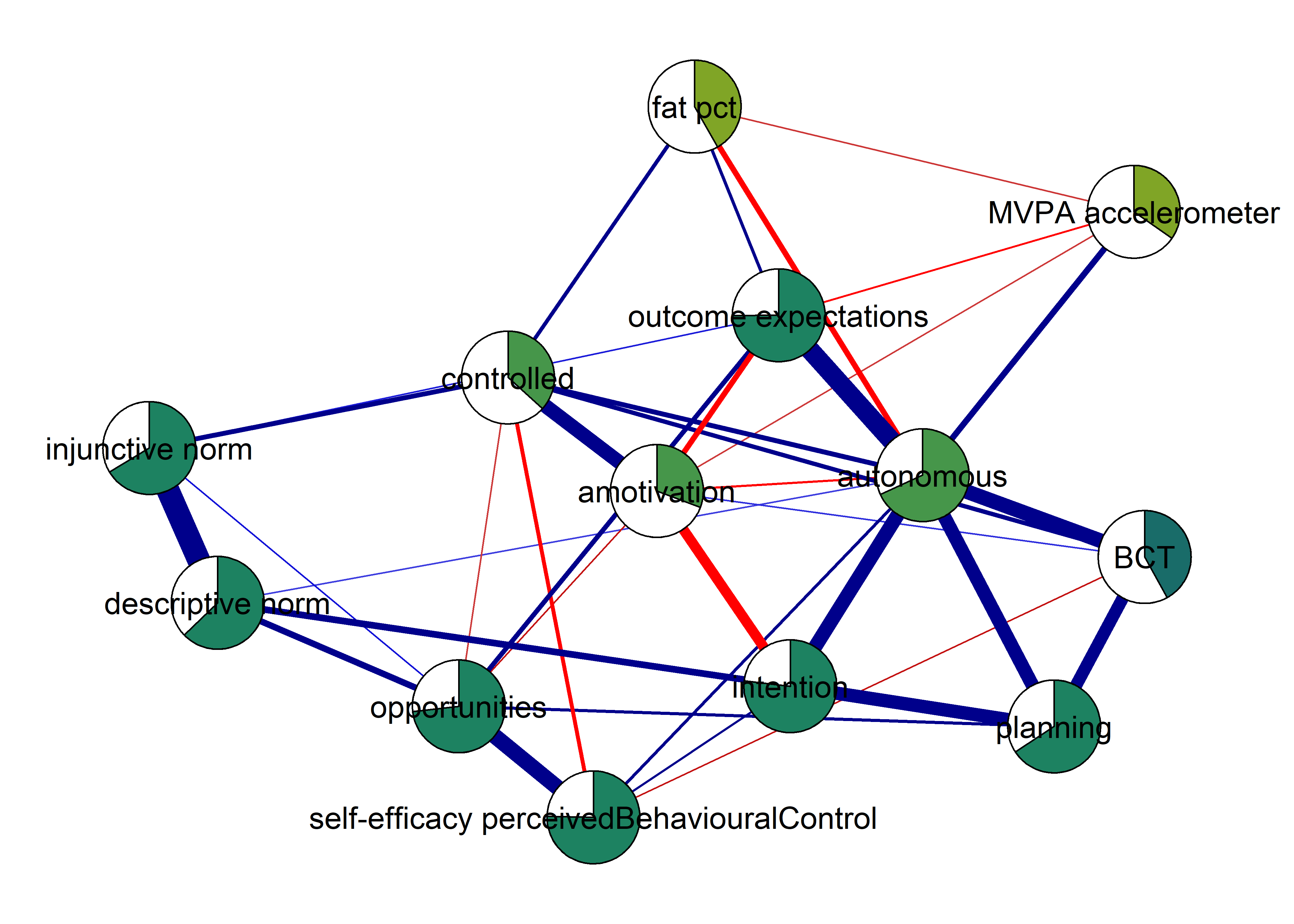
Centrality and stability
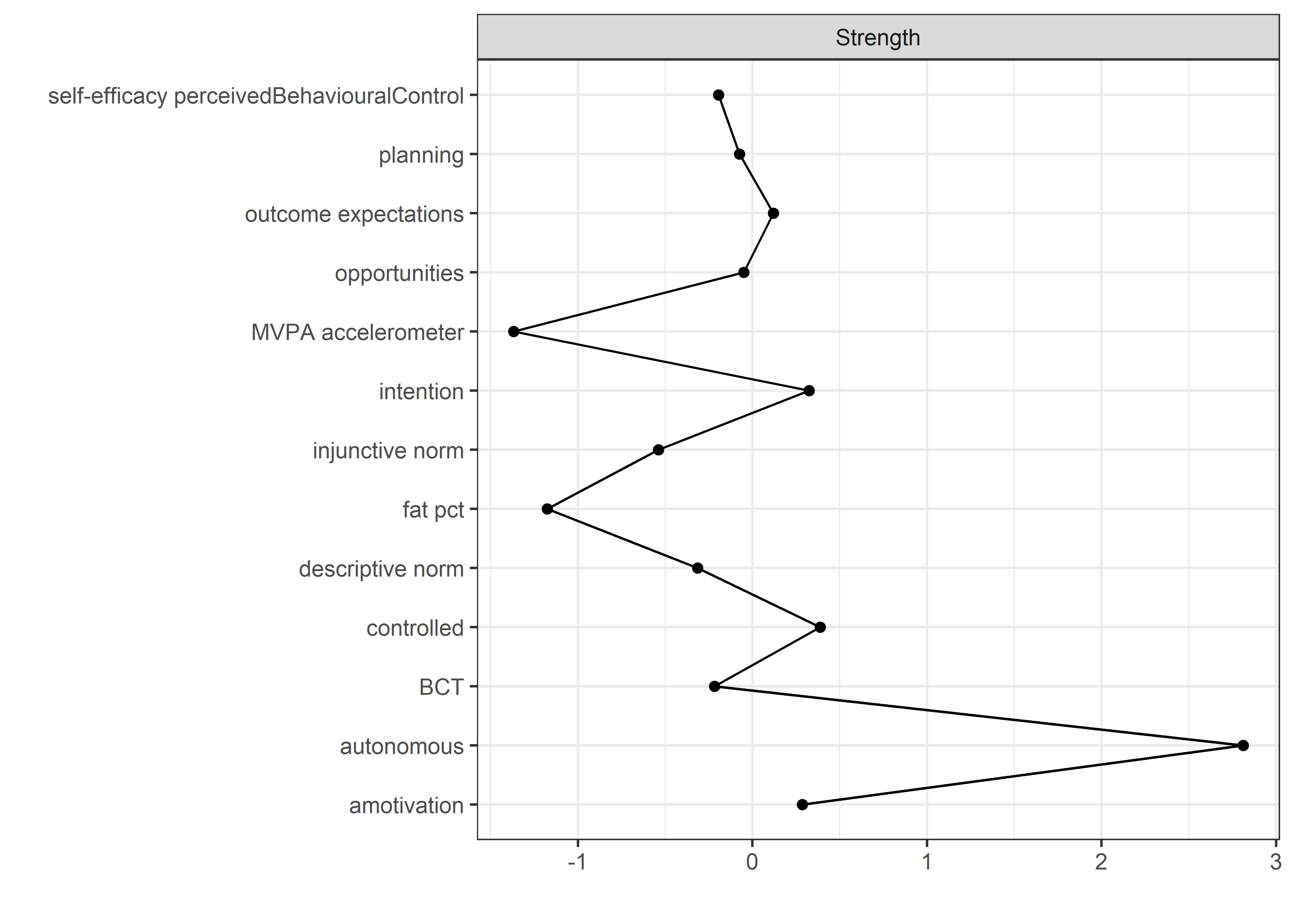
qgraph::centralityPlot(bootnetgraph,
               include = c("Strength", "ExpectedInfluence"),
               orderBy = "ExpectedInfluence")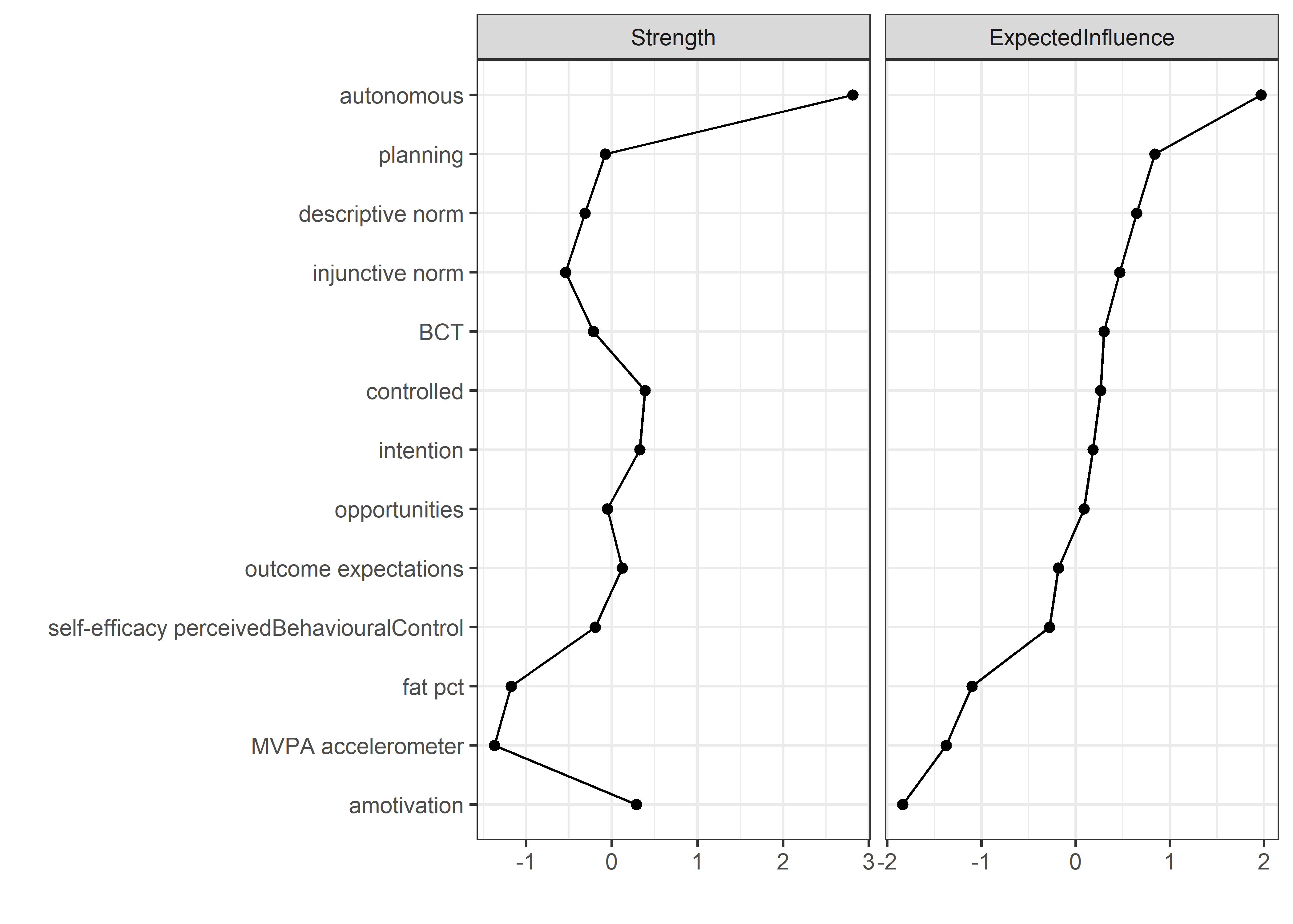
qgraph::centrality(bootnetgraph)$InDegree
##                        MVPA accelerometer
##                                 0.4219556
##                                  planning
##                                 0.8819272
##                                       BCT
##                                 0.8315025
##                               amotivation
##                                 1.0103095
##                                autonomous
##                                 1.9082304
##                                controlled
##                                 1.0466690
##                          descriptive norm
##                                 0.7969049
##                                   fat pct
##                                 0.4909482
##                           injunctive norm
##                                 0.7170571
##                                 intention
##                                 1.0241657
##                      outcome expectations
##                                 0.9513261
##                             opportunities
##                                 0.8908195
## self-efficacy perceivedBehaviouralControl
##                                 0.8397455
scale(qgraph::centrality(bootnetgraph)$InDegree)
##                                                  [,1]
## MVPA accelerometer                        -1.36911160
## planning                                  -0.07499172
## BCT                                       -0.21686031
## amotivation                                0.28620909
## autonomous                                 2.81248977
## controlled                                 0.38850581
## descriptive norm                          -0.31420004
## fat pct                                   -1.17500244
## injunctive norm                           -0.53885016
## intention                                  0.32519320
## outcome expectations                       0.12026074
## opportunities                             -0.04997347
## self-efficacy perceivedBehaviouralControl -0.19366889
## attr(,"scaled:center")
## [1] 0.9085816
## attr(,"scaled:scale")
## [1] 0.355432
qgraph::centrality(bootnetgraph)$Closeness
##                        MVPA accelerometer
##                               0.006700290
##                                  planning
##                               0.009973783
##                                       BCT
##                               0.009072923
##                               amotivation
##                               0.009086420
##                                autonomous
##                               0.012090602
##                                controlled
##                               0.009804271
##                          descriptive norm
##                               0.008196141
##                                   fat pct
##                               0.007323929
##                           injunctive norm
##                               0.007676769
##                                 intention
##                               0.011089400
##                      outcome expectations
##                               0.010084209
##                             opportunities
##                               0.008227697
## self-efficacy perceivedBehaviouralControl
##                               0.008207229
qgraph::centrality(bootnetgraph)$Betweenness
##                        MVPA accelerometer
##                                         0
##                                  planning
##                                         2
##                                       BCT
##                                         0
##                               amotivation
##                                         2
##                                autonomous
##                                        44
##                                controlled
##                                        12
##                          descriptive norm
##                                        12
##                                   fat pct
##                                         0
##                           injunctive norm
##                                         2
##                                 intention
##                                        24
##                      outcome expectations
##                                         6
##                             opportunities
##                                         6
## self-efficacy perceivedBehaviouralControl
##                                         2

cor(qgraph::centrality(bootnetgraph)$InDegree, qgraph::centrality(bootnetgraph)$Betweenness,
    method = "spearman")
## [1] 0.7614282

# bootnet_stability_determinants <- bootnet::bootnet(determinants_ggm_network, stepwise = FALSE, nBoots=1000)
# save(bootnet_stability_determinants, file = "./Rdata_files/bootnet_stability_determinants.Rdata")
load("./Rdata_files/bootnet_stability_determinants.Rdata")

plot(bootnet_stability_determinants, labels = TRUE, order = "sample") 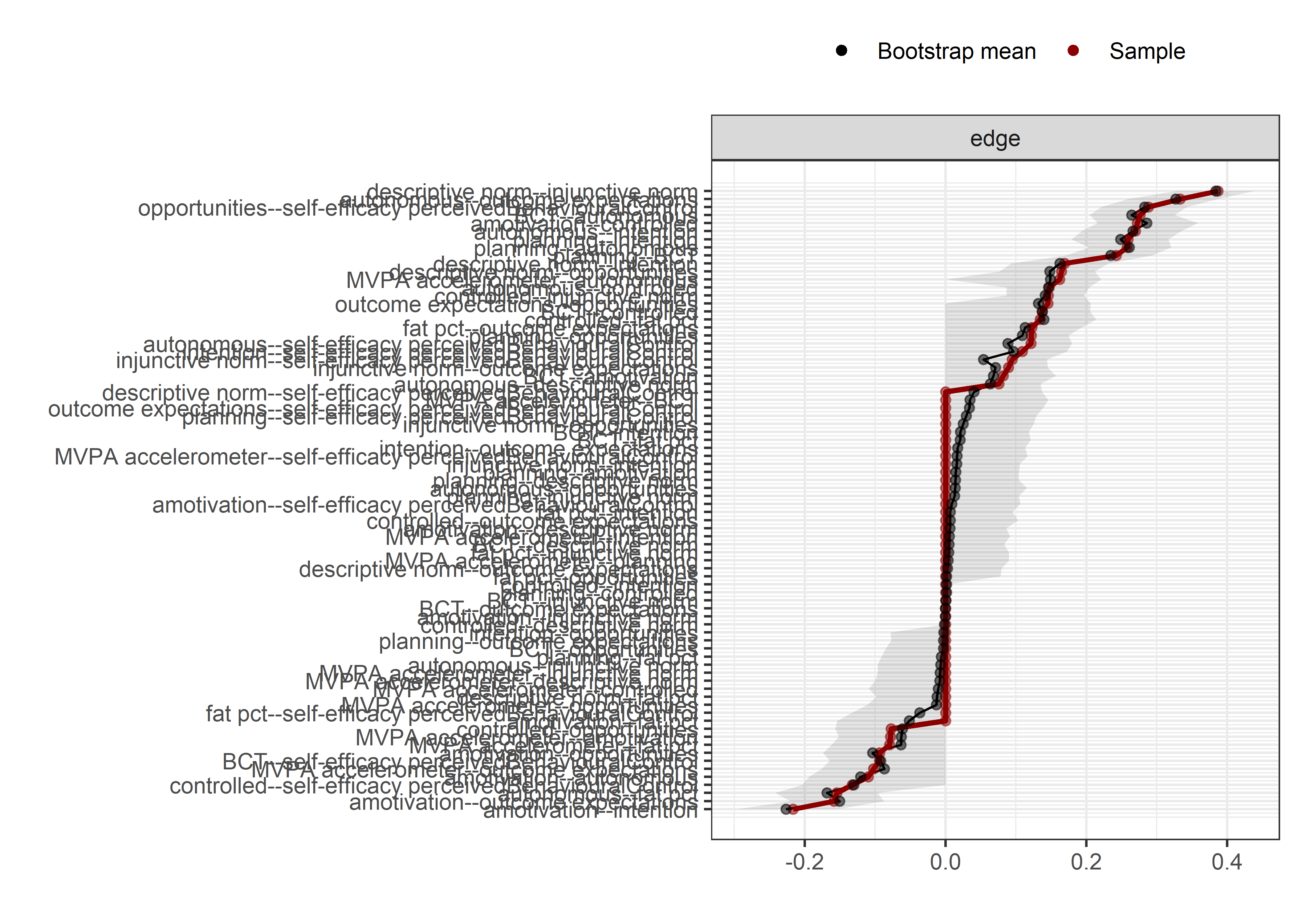
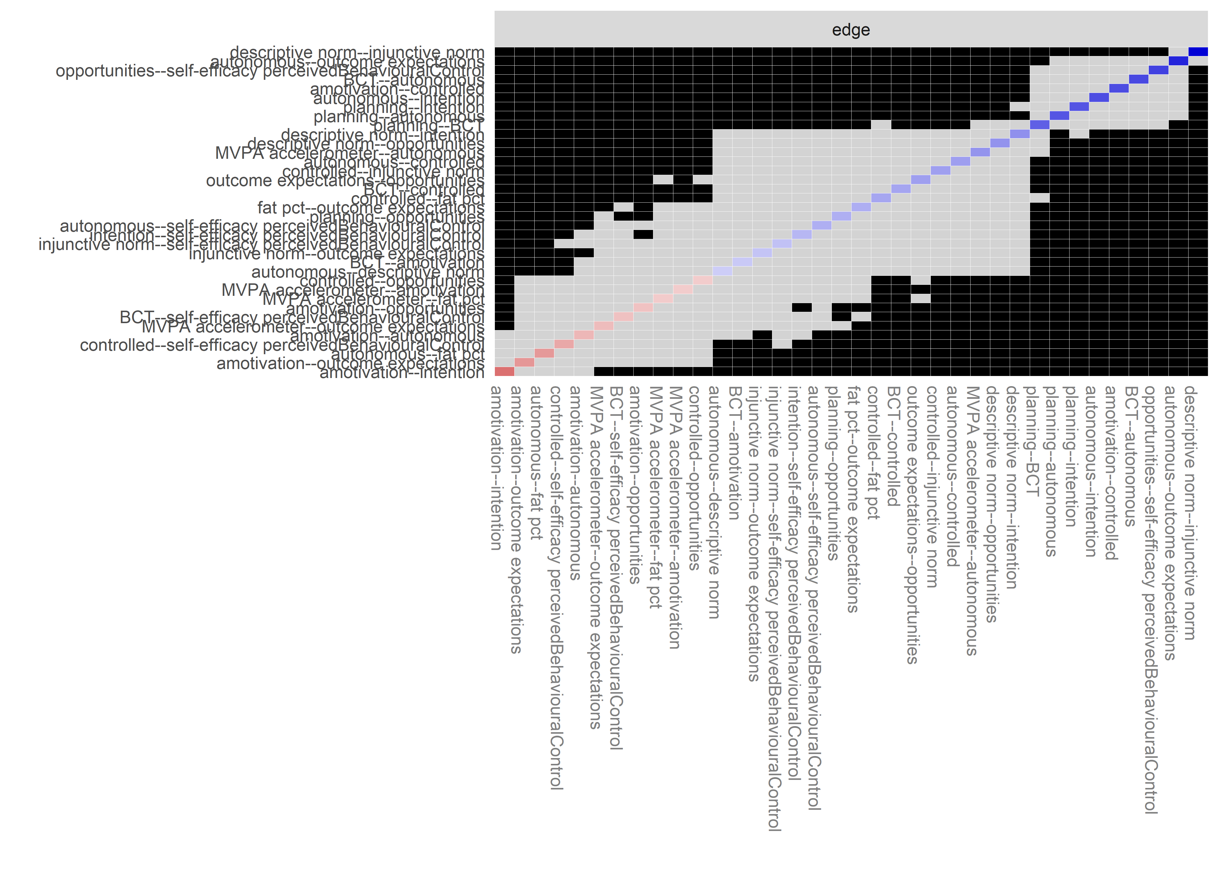
# bootnet_centrality_stability_determinants <- bootnet::bootnet(determinants_bootnet, stepwise = FALSE, nBoots=1000,nCores=8, type="case")
# save(bootnet_centrality_stability_determinants, file = "./Rdata_files/bootnet_centrality_stability_determinants.Rdata")
# load("./Rdata_files/bootnet_centrality_stability_determinants.Rdata")
#
# plot(bootnet_centrality_stability_determinants)
# plot(bootnet_centrality_stability_determinants, perNode=T, "strength")
#
# bootnet::corStability(bootnet_centrality_stability_determinants)
# boot2 <- bootnet::bootnet(Network1, stepwise = FALSE, nBoots = 2500, type = "case", nCores = 2)
# bootnet::corStability(boot2)
#
# plot(boot2)
#
# differenceTest(boot1, "auton", "intent", measure = c("strength", "closeness", "betweenness"))
#
# plot(boot1, "edge", plot = "difference", onlyNonZero = TRUE, order = "sample")
#
# plot(boot1, "strength")
# plot(boot1, "betweenness")
# plot(boot1, "closeness")PA motivation examined
Motivation correlation matrix
regulations.df <- df %>% dplyr::select(
  mvpaAccelerometer_T1,
  padaysLastweek_T1,
  PA_amotivation_02_T1,
  PA_amotivation_01_T1,
  PA_amotivation_03_T1,
  PA_amotivation_04_T1,
  PA_extrinsic_01_T1,
  PA_extrinsic_02_T1,
  PA_extrinsic_03_T1,
  PA_introjected_01_T1,
  PA_introjected_02_T1,
  PA_identified_01_T1,
  PA_identified_02_T1,
  PA_identified_03_T1,
  PA_integrated_01_T1,
  PA_integrated_02_T1,
  PA_integrated_03_T1,
  PA_intrinsic_01_T1,
  PA_intrinsic_02_T1,
  PA_intrinsic_03_T1,
  Autonomous_sumscore = PA_autonomous_T1,
  Controlled_sumscore = PA_controlled_T1,
  weartimeAccelerometer_T1) %>%
  mutate(mvpaAccelerometer_percentageWeartime_T1 = mvpaAccelerometer_T1 / weartimeAccelerometer_T1)

# Create a covariance matrix of the data
covMatrix <- regulations.df %>% cov(use = "pairwise.complete.obs")

# Transform the matrix so, that lower diagonal of the matrix shows partial correlations,
# while the upper one shows bivariate correlations.
matrix_corLower_parcorUpper <- covMatrix %>% ggm::correlations()

# Show the matrix
matrix_corLower_parcorUpper %>% papaja::apa_table(caption = "Correlation matrix of key variables of interest. Lower diagonal shows bivariate correlations, upper diagonal shows partial correlations")| mvpaAccelerometer_T1 | padaysLastweek_T1 | PA_amotivation_02_T1 | PA_amotivation_01_T1 | PA_amotivation_03_T1 | PA_amotivation_04_T1 | PA_extrinsic_01_T1 | PA_extrinsic_02_T1 | PA_extrinsic_03_T1 | PA_introjected_01_T1 | PA_introjected_02_T1 | PA_identified_01_T1 | PA_identified_02_T1 | PA_identified_03_T1 | PA_integrated_01_T1 | PA_integrated_02_T1 | PA_integrated_03_T1 | PA_intrinsic_01_T1 | PA_intrinsic_02_T1 | PA_intrinsic_03_T1 | Autonomous_sumscore | Controlled_sumscore | weartimeAccelerometer_T1 | mvpaAccelerometer_percentageWeartime_T1 | |
|---|---|---|---|---|---|---|---|---|---|---|---|---|---|---|---|---|---|---|---|---|---|---|---|---|
| mvpaAccelerometer_T1 | 1.00 | 0.11 | 0.02 | -0.01 | -0.02 | -0.02 | -0.03 | -0.05 | -0.05 | -0.05 | -0.05 | 0.01 | -0.01 | 0.03 | 0.06 | 0.01 | 0.00 | 0.04 | -0.01 | 0.06 | -0.03 | 0.05 | 0.90 | 1.00 |
| padaysLastweek_T1 | 0.29 | 1.00 | 0.01 | 0.03 | -0.02 | 0.05 | -0.04 | -0.01 | -0.03 | -0.03 | -0.02 | -0.01 | -0.01 | 0.03 | -0.01 | -0.02 | 0.03 | -0.04 | 0.00 | 0.03 | 0.02 | 0.03 | -0.11 | -0.09 |
| PA_amotivation_02_T1 | -0.15 | -0.11 | 1.00 | 0.33 | 0.23 | 0.13 | 0.00 | 0.03 | 0.04 | 0.00 | 0.02 | -0.02 | -0.02 | -0.02 | -0.04 | -0.01 | -0.04 | -0.05 | -0.02 | -0.01 | 0.03 | -0.01 | -0.04 | -0.03 |
| PA_amotivation_01_T1 | -0.17 | -0.13 | 0.59 | 1.00 | 0.13 | 0.15 | 0.03 | 0.01 | 0.05 | 0.02 | 0.00 | -0.02 | -0.03 | -0.03 | 0.00 | -0.05 | -0.03 | -0.03 | -0.02 | -0.04 | 0.03 | -0.02 | 0.03 | 0.01 |
| PA_amotivation_03_T1 | -0.08 | -0.11 | 0.57 | 0.54 | 1.00 | 0.47 | 0.04 | 0.02 | 0.02 | 0.02 | 0.01 | -0.04 | -0.09 | -0.01 | 0.01 | -0.03 | 0.00 | -0.03 | -0.07 | -0.07 | 0.04 | -0.02 | 0.03 | 0.02 |
| PA_amotivation_04_T1 | -0.10 | -0.06 | 0.53 | 0.52 | 0.69 | 1.00 | 0.00 | 0.01 | 0.02 | -0.01 | 0.01 | 0.01 | -0.04 | -0.01 | -0.02 | 0.04 | 0.03 | -0.01 | -0.01 | 0.06 | -0.01 | 0.00 | 0.02 | 0.02 |
| PA_extrinsic_01_T1 | -0.05 | -0.07 | 0.28 | 0.29 | 0.27 | 0.27 | 1.00 | -0.80 | -0.83 | -0.89 | -0.89 | 0.56 | 0.53 | 0.51 | 0.53 | 0.48 | 0.51 | 0.50 | 0.51 | 0.48 | -0.61 | 0.93 | 0.04 | 0.02 |
| PA_extrinsic_02_T1 | -0.03 | 0.00 | 0.29 | 0.26 | 0.26 | 0.28 | 0.63 | 1.00 | -0.80 | -0.87 | -0.88 | 0.55 | 0.53 | 0.52 | 0.53 | 0.48 | 0.53 | 0.51 | 0.51 | 0.46 | -0.61 | 0.92 | 0.06 | 0.04 |
| PA_extrinsic_03_T1 | -0.07 | -0.04 | 0.35 | 0.33 | 0.29 | 0.32 | 0.59 | 0.61 | 1.00 | -0.88 | -0.89 | 0.55 | 0.54 | 0.51 | 0.54 | 0.48 | 0.54 | 0.51 | 0.53 | 0.46 | -0.62 | 0.93 | 0.05 | 0.04 |
| PA_introjected_01_T1 | 0.02 | 0.09 | 0.05 | 0.00 | 0.01 | 0.02 | 0.27 | 0.32 | 0.30 | 1.00 | -0.87 | 0.56 | 0.53 | 0.52 | 0.53 | 0.48 | 0.51 | 0.52 | 0.51 | 0.47 | -0.62 | 0.96 | 0.06 | 0.04 |
| PA_introjected_02_T1 | 0.01 | 0.13 | 0.02 | -0.05 | -0.03 | 0.00 | 0.21 | 0.25 | 0.23 | 0.69 | 1.00 | 0.59 | 0.55 | 0.54 | 0.56 | 0.50 | 0.55 | 0.55 | 0.53 | 0.48 | -0.64 | 0.96 | 0.05 | 0.04 |
| PA_identified_01_T1 | 0.11 | 0.27 | -0.19 | -0.22 | -0.23 | -0.20 | -0.01 | 0.01 | -0.01 | 0.25 | 0.31 | 1.00 | -0.70 | -0.71 | -0.75 | -0.73 | -0.73 | -0.74 | -0.76 | -0.68 | 0.90 | -0.59 | -0.03 | 0.00 |
| PA_identified_02_T1 | 0.08 | 0.28 | -0.30 | -0.32 | -0.38 | -0.35 | -0.10 | -0.07 | -0.07 | 0.20 | 0.25 | 0.61 | 1.00 | -0.68 | -0.72 | -0.73 | -0.73 | -0.68 | -0.73 | -0.63 | 0.87 | -0.57 | -0.02 | 0.01 |
| PA_identified_03_T1 | 0.24 | 0.42 | -0.27 | -0.31 | -0.25 | -0.23 | -0.11 | -0.05 | -0.08 | 0.22 | 0.27 | 0.55 | 0.61 | 1.00 | -0.61 | -0.64 | -0.64 | -0.62 | -0.69 | -0.61 | 0.82 | -0.55 | -0.04 | -0.02 |
| PA_integrated_01_T1 | 0.23 | 0.37 | -0.23 | -0.25 | -0.18 | -0.18 | -0.05 | -0.01 | -0.01 | 0.22 | 0.29 | 0.48 | 0.53 | 0.74 | 1.00 | -0.59 | -0.67 | -0.65 | -0.72 | -0.64 | 0.84 | -0.57 | -0.07 | -0.05 |
| PA_integrated_02_T1 | 0.21 | 0.37 | -0.23 | -0.28 | -0.20 | -0.16 | -0.07 | -0.01 | -0.02 | 0.22 | 0.27 | 0.48 | 0.52 | 0.71 | 0.74 | 1.00 | -0.62 | -0.60 | -0.66 | -0.64 | 0.82 | -0.51 | -0.02 | 0.00 |
| PA_integrated_03_T1 | 0.30 | 0.44 | -0.23 | -0.27 | -0.19 | -0.14 | -0.11 | -0.04 | -0.03 | 0.13 | 0.20 | 0.48 | 0.51 | 0.70 | 0.67 | 0.71 | 1.00 | -0.73 | -0.66 | -0.50 | 0.84 | -0.56 | -0.02 | 0.01 |
| PA_intrinsic_01_T1 | 0.20 | 0.35 | -0.32 | -0.35 | -0.31 | -0.27 | -0.13 | -0.08 | -0.09 | 0.26 | 0.31 | 0.49 | 0.61 | 0.72 | 0.68 | 0.72 | 0.64 | 1.00 | -0.62 | -0.52 | 0.82 | -0.55 | -0.05 | -0.03 |
| PA_intrinsic_02_T1 | 0.21 | 0.38 | -0.30 | -0.32 | -0.32 | -0.25 | -0.15 | -0.10 | -0.07 | 0.13 | 0.17 | 0.45 | 0.55 | 0.66 | 0.60 | 0.67 | 0.72 | 0.73 | 1.00 | -0.52 | 0.85 | -0.55 | -0.01 | 0.01 |
| PA_intrinsic_03_T1 | 0.20 | 0.41 | -0.27 | -0.31 | -0.29 | -0.20 | -0.14 | -0.10 | -0.09 | 0.15 | 0.19 | 0.47 | 0.58 | 0.68 | 0.62 | 0.66 | 0.77 | 0.74 | 0.79 | 1.00 | 0.76 | -0.50 | -0.08 | -0.06 |
| Autonomous_sumscore | 0.24 | 0.45 | -0.31 | -0.35 | -0.31 | -0.27 | -0.12 | -0.06 | -0.06 | 0.24 | 0.31 | 0.68 | 0.75 | 0.86 | 0.82 | 0.84 | 0.84 | 0.86 | 0.84 | 0.85 | 1.00 | 0.66 | 0.05 | 0.02 |
| Controlled_sumscore | -0.02 | 0.05 | 0.24 | 0.19 | 0.19 | 0.21 | 0.69 | 0.71 | 0.69 | 0.78 | 0.72 | 0.18 | 0.09 | 0.11 | 0.15 | 0.14 | 0.06 | 0.12 | 0.03 | 0.04 | 0.13 | 1.00 | -0.06 | -0.04 |
| weartimeAccelerometer_T1 | 0.15 | -0.04 | 0.02 | 0.08 | 0.07 | 0.06 | 0.05 | 0.05 | 0.04 | 0.01 | -0.06 | -0.06 | -0.07 | -0.01 | -0.01 | -0.01 | -0.01 | -0.03 | 0.00 | -0.03 | -0.03 | 0.02 | 1.00 | -0.90 |
| mvpaAccelerometer_percentageWeartime_T1 | 0.98 | 0.29 | -0.15 | -0.18 | -0.10 | -0.11 | -0.07 | -0.04 | -0.08 | 0.02 | 0.03 | 0.12 | 0.09 | 0.24 | 0.23 | 0.22 | 0.30 | 0.20 | 0.22 | 0.20 | 0.25 | -0.02 | -0.03 | 1.00 |
labs <- names(regulations.df)
# Plot the matrix as a correlogram
matrix_corLower_parcorUpper %>% corrgram::corrgram(
  type = "cor",
  lower.panel = corrgram::panel.pie,
  upper.panel = corrgram::panel.pie,
  outer.labels = list(bottom = list(labels = labs, cex = 0.75, srt = 30),
                      left = list(labels = labs, cex = 0.75, srt = 30)),
  main = "Bivariate (upper diagonal) and partial (lower diagonal)\ncorrelations of BCTs, motivation and self-reported MVPA")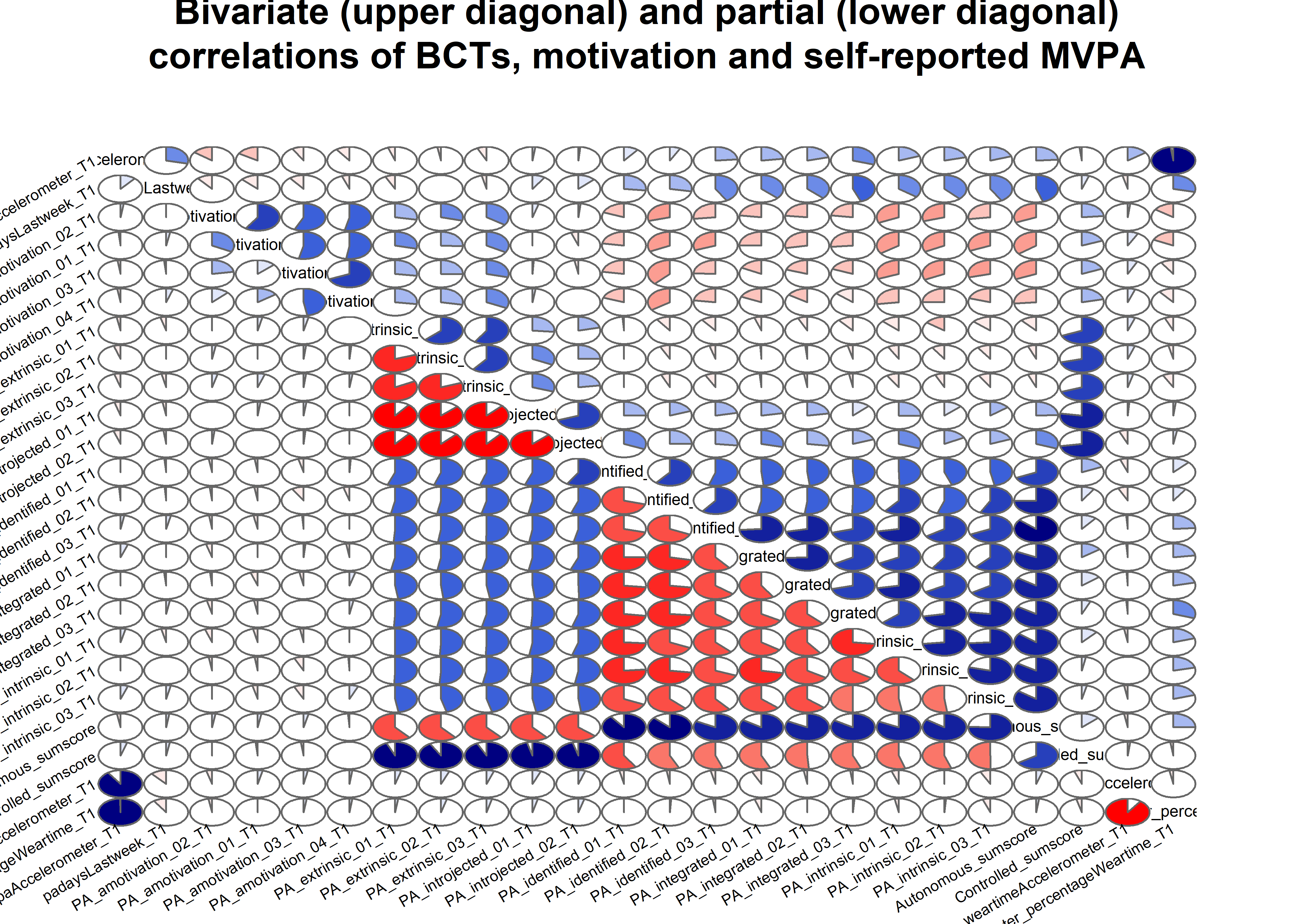
corMatrix_motivations <- regulations.df %>% cor(use = "pairwise.complete.obs", method = "spearman")

variableNames <- labels(corMatrix_motivations)[[1]] # Extract list of variable names to use in the next call

corMatrix_motivations %>%
  as.data.frame(.) %>%
  dplyr::mutate(Variable = variableNames) %>%
  dplyr::select(Variable,
                `MVPA accelerometer` = mvpaAccelerometer_T1, `MVPA self report` = padaysLastweek_T1,
                `MVPA accelerometer (% weartime)` = mvpaAccelerometer_percentageWeartime_T1,
                `Accelerometer wear time` = weartimeAccelerometer_T1) %>%
  dplyr::arrange(desc(`MVPA accelerometer`)) %>%
  DT::datatable(caption = "Bivariate correlations between motivation and MVPA. Sorted by correlation strength with MVPA accelerometer.")
corMatrix_motivations %>%
  as.data.frame(.) %>%
  dplyr::transmute(Variable = variableNames,
                   "Accelerometer minus self-report" = mvpaAccelerometer_T1 - padaysLastweek_T1,
                   "Accelerometer minus accelerometer-as-%-weartime" = mvpaAccelerometer_T1 - mvpaAccelerometer_percentageWeartime_T1) %>%
  dplyr::arrange(desc(`Accelerometer minus self-report`)) %>%
  DT::datatable(caption = "Differences in correlations among the measures")
Motivational regulations network
## TEE TĂNNE PIEFILL? tummempi sama väri tai opacity?
# Was going to do fused graphical lasso, but the items not normal...
# s1 <- regulations.df %>% filter(school == 1) %>% dplyr::select(6:ncol(regulations.df)) # %>% na.omit(.)
# s2 <- regulations.df %>% filter(school == 2) %>% dplyr::select(6:ncol(regulations.df)) # %>% na.omit(.)
# s3 <- regulations.df %>% filter(school == 3) %>% dplyr::select(6:ncol(regulations.df)) # %>% na.omit(.)
# s4 <- regulations.df %>% filter(school == 4) %>% dplyr::select(6:ncol(regulations.df)) # %>% na.omit(.)
# s5 <- regulations.df %>% filter(school == 5) %>% dplyr::select(6:ncol(regulations.df)) # %>% na.omit(.)
#
# network2 <- EstimateGroupNetwork(list("1" = s1,
# "2" = s2,
# "3" = s3,
# "4" = s4,
# "5" = s5),
# n = c(nrow(s1), nrow(s2), nrow(s3), nrow(s4), nrow(s5)))
#
regulations.df <- df %>% dplyr::select(
id,
intervention,
group,
school,
girl,
PA_amotivation_02_T1,
PA_amotivation_01_T1,
PA_amotivation_03_T1,
PA_amotivation_04_T1,
PA_extrinsic_01_T1,
PA_extrinsic_02_T1,
PA_extrinsic_03_T1,
PA_introjected_01_T1,
PA_introjected_02_T1,
PA_identified_01_T1,
PA_identified_02_T1,
PA_identified_03_T1,
PA_integrated_01_T1,
PA_integrated_02_T1,
PA_integrated_03_T1,
PA_intrinsic_01_T1,
PA_intrinsic_02_T1,
PA_intrinsic_03_T1)
regulations.df <- regulations.df %>% mutate(
PA_amotivation_02_T1 = ifelse(PA_amotivation_02_T1 == 1, 0, 1),
PA_amotivation_01_T1 = ifelse(PA_amotivation_01_T1 == 1, 0, 1),
PA_amotivation_03_T1 = ifelse(PA_amotivation_03_T1 == 1, 0, 1),
PA_amotivation_04_T1 = ifelse(PA_amotivation_04_T1 == 1, 0, 1),
PA_extrinsic_01_T1 = ifelse(PA_extrinsic_01_T1 == 1, 0, 1),
PA_extrinsic_02_T1 = ifelse(PA_extrinsic_02_T1 == 1, 0, 1),
PA_extrinsic_03_T1 = ifelse(PA_extrinsic_03_T1 == 1, 0, 1),
PA_introjected_01_T1 = ifelse(PA_introjected_01_T1 == 1, 0, 1),
PA_introjected_02_T1 = ifelse(PA_introjected_02_T1 == 1, 0, 1),
PA_identified_01_T1 = ifelse(PA_identified_01_T1 == 1, 0, 1),
PA_identified_02_T1 = ifelse(PA_identified_02_T1 == 1, 0, 1),
PA_identified_03_T1 = ifelse(PA_identified_03_T1 == 1, 0, 1),
PA_integrated_01_T1 = ifelse(PA_integrated_01_T1 == 1, 0, 1),
PA_integrated_02_T1 = ifelse(PA_integrated_02_T1 == 1, 0, 1),
PA_integrated_03_T1 = ifelse(PA_integrated_03_T1 == 1, 0, 1),
PA_intrinsic_01_T1 = ifelse(PA_intrinsic_01_T1 == 1, 0, 1),
PA_intrinsic_02_T1 = ifelse(PA_intrinsic_02_T1 == 1, 0, 1),
PA_intrinsic_03_T1 = ifelse(PA_intrinsic_03_T1 == 1, 0, 1))
### GIRLS AND BOYS
S.boys <- regulations.df %>% filter(girl == "boy") %>% dplyr::select(6:ncol(regulations.df)) # %>% na.omit(.)
S.girls <- regulations.df %>% filter(girl == "girl") %>% dplyr::select(6:ncol(regulations.df)) # %>% na.omit(.)
nwBoys <- bootnet::estimateNetwork(S.boys, default="IsingFit")
##
|
| | 0%
|
|==== | 6%
|
|======= | 11%
|
|=========== | 17%
|
|============== | 22%
|
|================== | 28%
|
|====================== | 33%
|
|========================= | 39%
|
|============================= | 44%
|
|================================ | 50%
|
|==================================== | 56%
|
|======================================== | 61%
|
|=========================================== | 67%
|
|=============================================== | 72%
|
|=================================================== | 78%
|
|====================================================== | 83%
|
|========================================================== | 89%
|
|============================================================= | 94%
|
|=================================================================| 100%
nwGirls <- bootnet::estimateNetwork(S.girls, default="IsingFit")
##
|
| | 0%
|
|==== | 6%
|
|======= | 11%
|
|=========== | 17%
|
|============== | 22%
|
|================== | 28%
|
|====================== | 33%
|
|========================= | 39%
|
|============================= | 44%
|
|================================ | 50%
|
|==================================== | 56%
|
|======================================== | 61%
|
|=========================================== | 67%
|
|=============================================== | 72%
|
|=================================================== | 78%
|
|====================================================== | 83%
|
|========================================================== | 89%
|
|============================================================= | 94%
|
|=================================================================| 100%
data1 <- regulations.df %>% dplyr::select(6:ncol(regulations.df))
names(data1) <- c(paste0(rep("Amoti", 4), 1:4),
paste0(rep("Extri", 3), 1:3),
paste0(rep("Intro", 2), 1:2),
paste0(rep("Ident", 3), 1:3),
paste0(rep("Integ", 3), 1:3),
paste0(rep("Intri", 3), 1:3))
nwAll <- bootnet::estimateNetwork(data1, default="IsingFit")
##
|
| | 0%
|
|==== | 6%
|
|======= | 11%
|
|=========== | 17%
|
|============== | 22%
|
|================== | 28%
|
|====================== | 33%
|
|========================= | 39%
|
|============================= | 44%
|
|================================ | 50%
|
|==================================== | 56%
|
|======================================== | 61%
|
|=========================================== | 67%
|
|=============================================== | 72%
|
|=================================================== | 78%
|
|====================================================== | 83%
|
|========================================================== | 89%
|
|============================================================= | 94%
|
|=================================================================| 100%
# Create means for filling nodes
# girlmeans <- regulations.df %>% group_by(girl) %>%
# summarise_at(vars(5:(5+nItems-1)),
# funs(mean(., na.rm = TRUE))) %>%
# filter(girl == "girl") %>%
# dplyr::select(-1)
#
# boymeans <- regulations.df %>% group_by(girl) %>%
# summarise_at(vars(5:(5+nItems-1)),
# funs(mean(., na.rm = TRUE))) %>%
# filter(girl == "boy") %>%
# dplyr::select(-1)
# Find average layout for comparability and plot graphs next to each other
Layout <- qgraph::averageLayout(nwGirls, nwBoys)
layout(t(1:2))
plot(nwGirls, layout = Layout, label.scale = FALSE, title = "Girls", label.cex = 0.5,
# pie = girlmeans,
color = "skyblue",
pieBorder = 1)
plot(nwBoys, layout = Layout, label.scale = FALSE, title = "Boys", label.cex = 0.5,
# pie = boymeans,
color = "skyblue",
pieBorder = 1)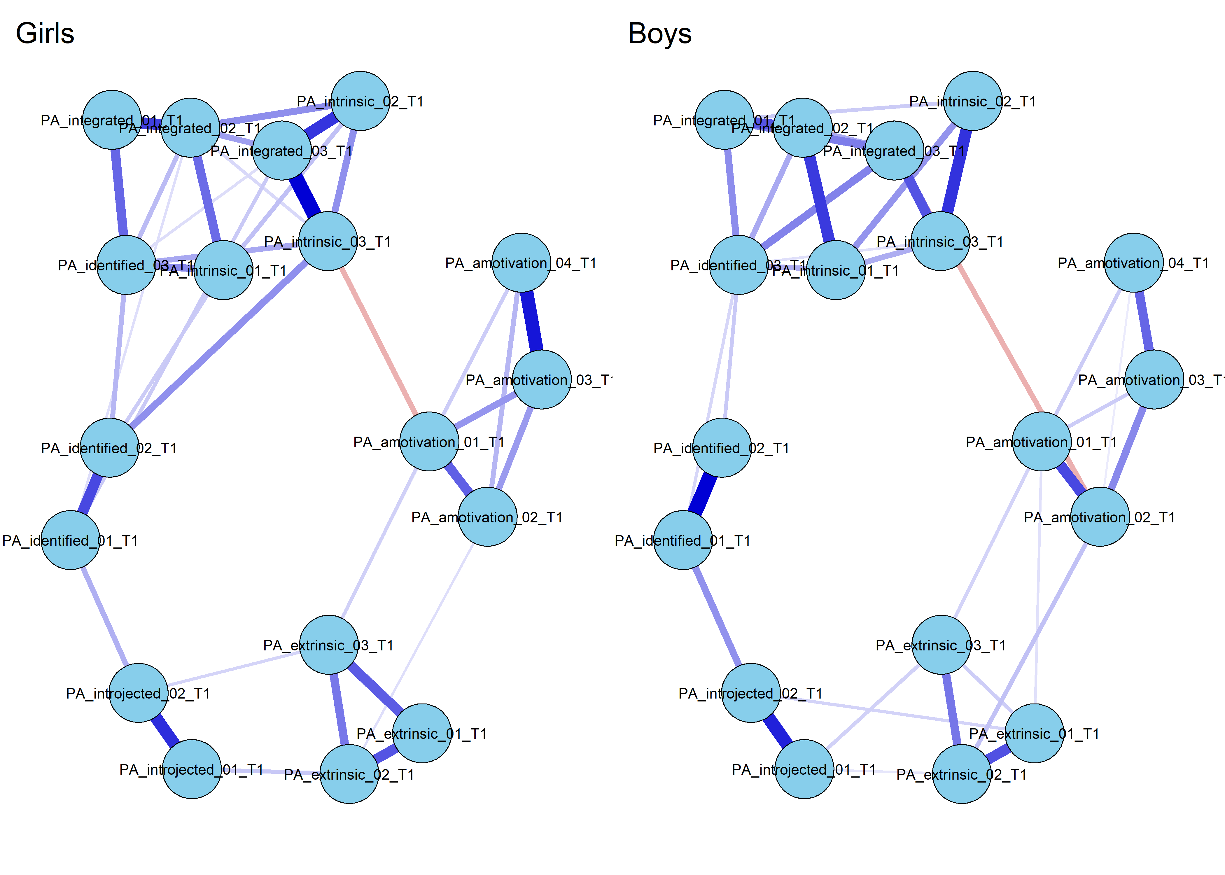
itemNames <- c('I can\'t see why I should bother exercising',
  'I do not see why I should have to exercise',
  ' I do not see the point in exercising',
  ' I think exercising is a waste of time',
  ' I exercise because other people say I should',
  ' I exercise because others will not be pleased with me if I do not',
  ' I feel under pressure from my friends/family to exercise',
  ' I feel guilty when I do not exercise',
  ' I feel like a failure when I have not exercised in a while',
  ' I think it is important to make the effort to exercise regularly',
  ' I value the benefits of exercise',
  ' it is important to me to exercise regularly',
  ' I exercise because it is consistent with my life goals.',
  ' I consider exercise consistent with my values.',
  ' I consider exercise a fundamental part of who I am.',
  ' I get pleasure and satisfaction from participating in exercise',
  ' I exercise because it is fun',
  ' I enjoy my exercise sessions')

itemGroups <- c(rep("Amotivation", 4),
                rep("Extrinsic", 3),
                rep("Introjected", 2),
                rep("Identified", 3),
                rep("Integrated", 3),
                rep("Intrinsic", 3))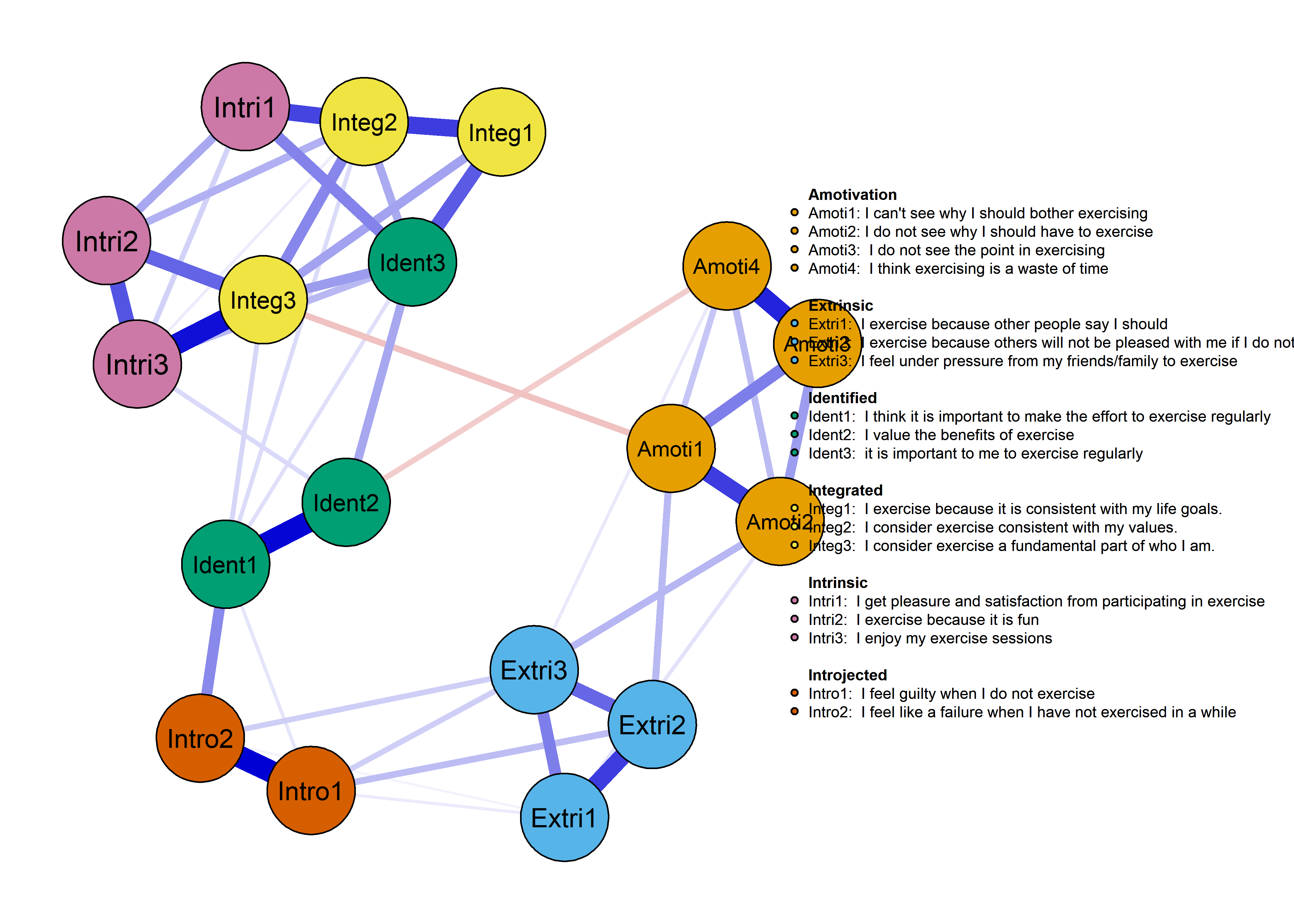
Session information
Description of the R environment can be found below.
devtools::session_info()
## - Session info ----------------------------------------------------------
## setting value
## version R version 3.6.0 (2019-04-26)
## os Windows 10 x64
## system x86_64, mingw32
## ui RTerm
## language (EN)
## collate Finnish_Finland.1252
## ctype Finnish_Finland.1252
## tz Europe/Helsinki
## date 2019-06-30
##
## - Packages --------------------------------------------------------------
## package * version date lib
## abind 1.4-5 2016-07-21 [1]
## acepack 1.4.1 2016-10-29 [1]
## assertthat 0.2.1 2019-03-21 [1]
## backports 1.1.4 2019-04-10 [1]
## base64enc 0.1-3 2015-07-28 [1]
## BayesFactor 0.9.12-4.2 2018-05-19 [1]
## bayesplot 1.7.0 2019-05-23 [1]
## BDgraph 2.59 2019-05-06 [1]
## BiasedUrn 1.07 2015-12-28 [1]
## bitops 1.0-6 2013-08-17 [1]
## boot 1.3-22 2019-04-02 [2]
## bootnet 1.2.2 2019-05-09 [1]
## brew 1.0-6 2011-04-13 [1]
## bridgesampling 0.6-0 2018-10-21 [1]
## brms * 2.8.0 2019-03-15 [1]
## brmstools * 0.5.3 2018-11-16 [1]
## Brobdingnag 1.2-6 2018-08-13 [1]
## broom 0.5.2 2019-04-07 [1]
## broom.mixed 0.2.4 2019-02-21 [1]
## broomExtra 0.0.3 2019-05-20 [1]
## callr 3.2.0 2019-03-15 [1]
## candisc 0.8-0 2017-09-19 [1]
## car 3.0-2 2018-08-23 [1]
## carData 3.0-2 2018-09-30 [1]
## caTools 1.17.1.2 2019-03-06 [1]
## cellranger 1.1.0 2016-07-27 [1]
## checkmate 1.9.3 2019-05-03 [1]
## cli 1.1.0 2019-03-19 [1]
## cluster 2.0.9 2019-05-01 [1]
## cmprsk 2.2-7 2014-06-17 [1]
## coda 0.19-2 2018-10-08 [1]
## codetools 0.2-16 2018-12-24 [2]
## coin 1.3-0 2019-03-08 [1]
## colorspace 1.4-1 2019-03-18 [1]
## colourpicker 1.0 2017-09-27 [1]
## corpcor 1.6.9 2017-04-01 [1]
## corrgram * 1.13 2018-07-09 [1]
## cowplot 0.9.4 2019-01-08 [1]
## crayon 1.3.4 2017-09-16 [1]
## crosstalk 1.0.0 2016-12-21 [1]
## curl 3.3 2019-01-10 [1]
## d3Network 0.5.2.1 2015-01-31 [1]
## data.table 1.12.2 2019-04-07 [1]
## data.tree 0.7.8 2018-09-24 [1]
## DBI 1.0.0 2018-05-02 [1]
## dendextend 1.12.0 2019-05-11 [1]
## DEoptimR 1.0-8 2016-11-19 [1]
## desc 1.2.0 2018-05-01 [1]
## DescTools 0.99.28 2019-03-17 [1]
## devtools 2.0.2 2019-04-08 [1]
## DiagrammeR 1.0.1 2019-04-22 [1]
## digest 0.6.19 2019-05-20 [1]
## diptest 0.75-7 2016-12-05 [1]
## downloader 0.4 2015-07-09 [1]
## dplyr * 0.8.1 2019-05-14 [1]
## DT 0.6 2019-05-09 [1]
## dygraphs 1.1.1.6 2018-07-11 [1]
## eigenmodel 1.10 2018-06-03 [1]
## ellipse 0.4.1 2018-01-05 [1]
## ellipsis 0.1.0 2019-02-19 [1]
## emmeans 1.3.4 2019-04-21 [1]
## EMT 1.1 2013-01-29 [1]
## Epi 2.37 2019-05-23 [1]
## estimability 1.3 2018-02-11 [1]
## etm 1.0.4 2018-07-11 [1]
## evaluate 0.14 2019-05-28 [1]
## expm 0.999-4 2019-03-21 [1]
## ez 4.4-0 2016-11-02 [1]
## fdrtool 1.2.15 2015-07-08 [1]
## fit.models 0.5-14 2017-04-06 [1]
## forcats * 0.4.0 2019-02-17 [1]
## foreach 1.4.4 2017-12-12 [1]
## foreign 0.8-71 2018-07-20 [1]
## Formula 1.2-3 2018-05-03 [1]
## fs 1.3.1 2019-05-06 [1]
## gclus 1.3.2 2019-01-07 [1]
## gdata 2.18.0 2017-06-06 [1]
## GeneNet 1.2.13 2015-08-02 [1]
## generics 0.0.2 2018-11-29 [1]
## GGally 1.4.0 2018-05-17 [1]
## ggcorrplot 0.1.3 2019-05-19 [1]
## ggExtra 0.8 2018-04-04 [1]
## ggm 2.3 2015-01-21 [1]
## ggplot2 * 3.1.1 2019-04-07 [1]
## ggrepel 0.8.1 2019-05-07 [1]
## ggridges * 0.5.1 2018-09-27 [1]
## ggsignif 0.5.0 2019-02-20 [1]
## ggstatsplot * 0.0.10 2019-03-17 [1]
## glasso 1.10 2018-07-13 [1]
## glmnet 2.0-18 2019-05-20 [1]
## glue 1.3.1 2019-03-12 [1]
## GPArotation 2014.11-1 2014-11-25 [1]
## gplots 3.0.1.1 2019-01-27 [1]
## gridExtra 2.3 2017-09-09 [1]
## groupedstats 0.0.6 2019-03-20 [1]
## gtable 0.3.0 2019-03-25 [1]
## gtools 3.8.1 2018-06-26 [1]
## haven 2.1.0 2019-02-19 [1]
## heplots 1.3-5 2018-04-03 [1]
## highr 0.8 2019-03-20 [1]
## Hmisc 4.2-0 2019-01-26 [1]
## hms 0.4.2 2018-03-10 [1]
## htmlTable 1.13.1 2019-01-07 [1]
## htmltools 0.3.6 2017-04-28 [1]
## htmlwidgets 1.3 2018-09-30 [1]
## httpuv 1.5.1 2019-04-05 [1]
## httr 1.4.0 2018-12-11 [1]
## huge 1.3.2 2019-04-08 [1]
## igraph 1.2.4.1 2019-04-22 [1]
## influenceR 0.1.0 2015-09-03 [1]
## inline 0.3.15 2018-05-18 [1]
## insight 0.3.0 2019-05-11 [1]
## IsingFit 0.3.1 2016-09-07 [1]
## IsingSampler 0.2 2015-03-02 [1]
## iterators 1.0.10 2018-07-13 [1]
## jmv 0.9.6.1 2019-04-22 [1]
## jmvcore 0.9.6.4 2019-03-28 [1]
## jomo 2.6-8 2019-05-21 [1]
## jpeg 0.1-8 2014-01-23 [1]
## jsonlite 1.6 2018-12-07 [1]
## KernSmooth 2.23-15 2015-06-29 [2]
## knitr * 1.23 2019-05-18 [1]
## labeling 0.3 2014-08-23 [1]
## later 0.8.0 2019-02-11 [1]
## lattice 0.20-38 2018-11-04 [2]
## latticeExtra 0.6-28 2016-02-09 [1]
## lavaan 0.6-3 2018-09-22 [1]
## lazyeval 0.2.2 2019-03-15 [1]
## libcoin 1.0-4 2019-02-28 [1]
## lme4 1.1-21 2019-03-05 [1]
## lmtest 0.9-37 2019-04-30 [1]
## longitudinal 1.1.12 2015-07-08 [1]
## loo 2.1.0 2019-03-13 [1]
## lubridate 1.7.4 2018-04-11 [1]
## magrittr 1.5 2014-11-22 [1]
## manipulate 1.0.1 2014-12-24 [1]
## markdown 1.0 2019-06-07 [1]
## MASS 7.3-51.4 2019-04-26 [1]
## Matrix 1.2-17 2019-03-22 [1]
## matrixcalc 1.0-3 2012-09-15 [1]
## MatrixModels 0.4-1 2015-08-22 [1]
## matrixStats 0.54.0 2018-07-23 [1]
## MBESS 4.5.1 2019-05-17 [1]
## mc2d 0.1-18 2017-03-06 [1]
## memoise 1.1.0 2017-04-21 [1]
## metafor 2.1-0 2019-05-14 [1]
## mgcv 1.8-28 2019-03-21 [1]
## mgm * 1.2-7 2019-05-09 [1]
## mice 3.5.0 2019-05-13 [1]
## mime 0.7 2019-06-11 [1]
## miniUI 0.1.1.1 2018-05-18 [1]
## minpack.lm 1.2-1 2016-11-20 [1]
## minqa 1.2.4 2014-10-09 [1]
## mitml 0.3-7 2019-01-07 [1]
## mitools 2.4 2019-04-26 [1]
## mnormt 1.5-5 2016-10-15 [1]
## modelr 0.1.4 2019-02-18 [1]
## modeltools 0.2-22 2018-07-16 [1]
## multcomp 1.4-10 2019-03-05 [1]
## multcompView 0.1-7 2015-07-31 [1]
## munsell 0.5.0 2018-06-12 [1]
## mvtnorm 1.0-10 2019-03-05 [1]
## NetworkComparisonTest * 2.0.1 2016-10-29 [1]
## NetworkToolbox 1.2.3 2019-01-31 [1]
## networktools 1.2.1 2019-05-20 [1]
## nlme 3.1-140 2019-05-12 [1]
## nloptr 1.2.1 2018-10-03 [1]
## nnet 7.3-12 2016-02-02 [2]
## nnls 1.4 2012-03-19 [1]
## nortest 1.0-4 2015-07-30 [1]
## numDeriv 2016.8-1.1 2019-06-06 [1]
## openxlsx 4.1.0.1 2019-05-28 [1]
## pacman * 0.5.1 2019-03-11 [1]
## paletteer 0.2.1 2019-02-13 [1]
## pan 1.6 2018-06-29 [1]
## pander 0.6.3 2018-11-06 [1]
## papaja * 0.1.0.9842 2018-11-18 [1]
## parcor 0.2-6 2014-09-04 [1]
## patchwork * 0.0.1 2018-11-21 [1]
## pbapply 1.4-0 2019-02-05 [1]
## pbivnorm 0.6.0 2015-01-23 [1]
## pcaPP 1.9-73 2018-01-14 [1]
## pillar 1.4.1 2019-05-28 [1]
## pkgbuild 1.0.3 2019-03-20 [1]
## pkgconfig 2.0.2 2018-08-16 [1]
## pkgload 1.0.2 2018-10-29 [1]
## plotrix 3.7-5 2019-04-07 [1]
## plyr 1.8.4 2016-06-08 [1]
## png 0.1-7 2013-12-03 [1]
## polynom 1.4-0 2019-03-22 [1]
## ppls 1.6-1.1 2018-07-20 [1]
## prettyunits 1.0.2 2015-07-13 [1]
## processx 3.3.1 2019-05-08 [1]
## promises 1.0.1 2018-04-13 [1]
## ps 1.3.0 2018-12-21 [1]
## psych 1.8.12 2019-01-12 [1]
## purrr * 0.3.2 2019-03-15 [1]
## purrrlyr 0.0.5 2019-03-15 [1]
## pwr 1.2-2 2018-03-03 [1]
## qgraph 1.6.2 2019-05-09 [1]
## R.methodsS3 1.7.1 2016-02-16 [1]
## R.oo 1.22.0 2018-04-22 [1]
## R.utils 2.8.0 2019-02-14 [1]
## R6 2.4.0 2019-02-14 [1]
## RColorBrewer 1.1-2 2014-12-07 [1]
## rcompanion 2.1.7 2019-04-09 [1]
## Rcpp * 1.0.1 2019-03-17 [1]
## readr * 1.3.1 2018-12-21 [1]
## readxl 1.3.1 2019-03-13 [1]
## registry 0.5-1 2019-03-05 [1]
## relaimpo 2.2-3 2018-03-10 [1]
## remotes 2.0.4 2019-04-10 [1]
## reshape 0.8.8 2018-10-23 [1]
## reshape2 1.4.3 2017-12-11 [1]
## rgexf 0.15.3 2015-03-24 [1]
## rio 0.5.16 2018-11-26 [1]
## rjson 0.2.20 2018-06-08 [1]
## rlang 0.3.4 2019-04-07 [1]
## rmarkdown 1.13 2019-05-22 [1]
## robust 0.4-18 2017-04-27 [1]
## robustbase 0.93-5 2019-05-12 [1]
## Rook 1.1-1 2014-10-20 [1]
## rpart 4.1-15 2019-04-12 [1]
## rprojroot 1.3-2 2018-01-03 [1]
## rrcov 1.4-7 2018-11-15 [1]
## rsconnect 0.8.13 2019-01-10 [1]
## rstan 2.18.2 2018-11-07 [1]
## rstantools 1.5.1 2018-08-22 [1]
## rstudioapi 0.10 2019-03-19 [1]
## rvest 0.3.4 2019-05-15 [1]
## sandwich 2.5-1 2019-04-06 [1]
## scales 1.0.0 2018-08-09 [1]
## SCRT 1.2.2 2018-03-07 [1]
## seriation 1.2-3 2018-02-05 [1]
## sessioninfo 1.1.1 2018-11-05 [1]
## shiny 1.3.2 2019-04-22 [1]
## shinyjs 1.0 2018-01-08 [1]
## shinystan 2.5.0 2018-05-01 [1]
## shinythemes 1.1.2 2018-11-06 [1]
## sjlabelled 1.0.17 2019-03-10 [1]
## sjmisc 2.7.9 2019-03-16 [1]
## sjstats 0.17.4 2019-03-15 [1]
## skimr 1.0.5 2019-02-25 [1]
## smacof 1.10-8 2018-06-14 [1]
## StanHeaders 2.18.1 2019-01-28 [1]
## stringi 1.4.3 2019-03-12 [1]
## stringr * 1.4.0 2019-02-10 [1]
## SuppDists 1.1-9.4 2016-09-23 [1]
## survey 3.36 2019-04-27 [1]
## survival 2.44-1.1 2019-04-01 [1]
## testthat 2.1.1 2019-04-23 [1]
## TH.data 1.0-10 2019-01-21 [1]
## threejs 0.3.1 2017-08-13 [1]
## tibble * 2.1.3 2019-06-06 [1]
## tidyr * 0.8.3 2019-03-01 [1]
## tidyselect 0.2.5 2018-10-11 [1]
## tidyverse * 1.2.1 2017-11-14 [1]
## TMB 1.7.15 2018-11-09 [1]
## TSP 1.1-7 2019-05-22 [1]
## userfriendlyscience 0.7.2 2018-09-24 [1]
## usethis 1.5.0 2019-04-07 [1]
## viridis 0.5.1 2018-03-29 [1]
## viridisLite 0.3.0 2018-02-01 [1]
## visNetwork 2.0.6 2019-03-26 [1]
## weights 1.0 2018-10-16 [1]
## whisker 0.3-2 2013-04-28 [1]
## withr 2.1.2 2018-03-15 [1]
## wordcloud 2.6 2018-08-24 [1]
## WRS2 0.10-0 2018-06-15 [1]
## xfun 0.7 2019-05-14 [1]
## XML 3.98-1.19 2019-03-06 [1]
## xml2 1.2.0 2018-01-24 [1]
## xtable 1.8-4 2019-04-21 [1]
## xts 0.11-2 2018-11-05 [1]
## yaml 2.2.0 2018-07-25 [1]
## zip 2.0.2 2019-05-13 [1]
## zoo 1.8-6 2019-05-28 [1]
## source
## CRAN (R 3.5.0)
## CRAN (R 3.5.0)
## CRAN (R 3.5.3)
## CRAN (R 3.5.3)
## CRAN (R 3.5.0)
## CRAN (R 3.5.0)
## CRAN (R 3.5.3)
## CRAN (R 3.5.3)
## CRAN (R 3.5.0)
## CRAN (R 3.5.0)
## CRAN (R 3.6.0)
## CRAN (R 3.5.3)
## CRAN (R 3.5.0)
## CRAN (R 3.5.1)
## CRAN (R 3.5.3)
## Github (mvuorre/brmstools@dc9c1dd)
## CRAN (R 3.5.1)
## CRAN (R 3.5.3)
## CRAN (R 3.5.1)
## CRAN (R 3.5.3)
## CRAN (R 3.5.3)
## CRAN (R 3.5.1)
## CRAN (R 3.5.1)
## CRAN (R 3.5.1)
## CRAN (R 3.5.3)
## CRAN (R 3.5.0)
## CRAN (R 3.5.3)
## CRAN (R 3.5.3)
## CRAN (R 3.5.3)
## CRAN (R 3.5.0)
## CRAN (R 3.5.1)
## CRAN (R 3.6.0)
## CRAN (R 3.5.3)
## CRAN (R 3.5.3)
## CRAN (R 3.5.0)
## CRAN (R 3.5.0)
## CRAN (R 3.5.1)
## CRAN (R 3.5.2)
## CRAN (R 3.5.0)
## CRAN (R 3.5.0)
## CRAN (R 3.5.2)
## CRAN (R 3.5.0)
## CRAN (R 3.5.3)
## CRAN (R 3.5.1)
## CRAN (R 3.5.0)
## CRAN (R 3.5.3)
## CRAN (R 3.5.0)
## CRAN (R 3.5.1)
## CRAN (R 3.5.3)
## CRAN (R 3.5.3)
## CRAN (R 3.5.3)
## CRAN (R 3.5.3)
## CRAN (R 3.5.0)
## CRAN (R 3.5.0)
## CRAN (R 3.5.3)
## CRAN (R 3.5.3)
## CRAN (R 3.5.1)
## CRAN (R 3.5.0)
## CRAN (R 3.5.0)
## CRAN (R 3.5.1)
## CRAN (R 3.5.3)
## CRAN (R 3.5.2)
## CRAN (R 3.5.3)
## CRAN (R 3.5.0)
## CRAN (R 3.5.1)
## CRAN (R 3.5.3)
## CRAN (R 3.5.3)
## CRAN (R 3.5.3)
## CRAN (R 3.5.0)
## CRAN (R 3.5.1)
## CRAN (R 3.5.2)
## CRAN (R 3.5.0)
## CRAN (R 3.5.1)
## CRAN (R 3.5.0)
## CRAN (R 3.5.3)
## CRAN (R 3.5.2)
## CRAN (R 3.5.0)
## CRAN (R 3.5.0)
## CRAN (R 3.5.1)
## CRAN (R 3.5.0)
## CRAN (R 3.5.3)
## CRAN (R 3.5.0)
## CRAN (R 3.5.0)
## CRAN (R 3.5.3)
## CRAN (R 3.5.3)
## CRAN (R 3.5.1)
## CRAN (R 3.5.2)
## CRAN (R 3.5.3)
## CRAN (R 3.5.1)
## CRAN (R 3.5.3)
## CRAN (R 3.5.3)
## CRAN (R 3.5.2)
## CRAN (R 3.5.2)
## CRAN (R 3.5.0)
## CRAN (R 3.5.3)
## CRAN (R 3.5.1)
## CRAN (R 3.5.0)
## CRAN (R 3.5.2)
## CRAN (R 3.5.1)
## CRAN (R 3.5.3)
## CRAN (R 3.5.2)
## CRAN (R 3.5.0)
## CRAN (R 3.5.2)
## CRAN (R 3.5.0)
## CRAN (R 3.5.1)
## CRAN (R 3.5.3)
## CRAN (R 3.5.1)
## CRAN (R 3.5.3)
## CRAN (R 3.5.3)
## CRAN (R 3.5.0)
## CRAN (R 3.5.0)
## CRAN (R 3.5.3)
## CRAN (R 3.5.1)
## CRAN (R 3.5.0)
## CRAN (R 3.5.1)
## CRAN (R 3.5.3)
## CRAN (R 3.5.3)
## CRAN (R 3.5.3)
## CRAN (R 3.5.0)
## CRAN (R 3.5.1)
## CRAN (R 3.6.0)
## CRAN (R 3.5.3)
## CRAN (R 3.5.0)
## CRAN (R 3.5.1)
## CRAN (R 3.6.0)
## CRAN (R 3.5.0)
## CRAN (R 3.5.2)
## CRAN (R 3.5.3)
## CRAN (R 3.5.3)
## CRAN (R 3.5.3)
## CRAN (R 3.5.3)
## CRAN (R 3.5.0)
## CRAN (R 3.5.3)
## CRAN (R 3.5.0)
## CRAN (R 3.5.0)
## CRAN (R 3.5.0)
## CRAN (R 3.5.3)
## CRAN (R 3.5.3)
## CRAN (R 3.5.3)
## CRAN (R 3.5.0)
## CRAN (R 3.5.0)
## CRAN (R 3.5.1)
## CRAN (R 3.5.3)
## CRAN (R 3.5.0)
## CRAN (R 3.5.0)
## CRAN (R 3.5.3)
## CRAN (R 3.5.3)
## Github (jmbh/mgm@029ab66)
## CRAN (R 3.5.3)
## CRAN (R 3.5.3)
## CRAN (R 3.5.0)
## CRAN (R 3.5.0)
## CRAN (R 3.5.0)
## CRAN (R 3.5.2)
## CRAN (R 3.5.3)
## CRAN (R 3.5.0)
## CRAN (R 3.5.1)
## CRAN (R 3.5.1)
## CRAN (R 3.5.3)
## CRAN (R 3.5.0)
## CRAN (R 3.5.0)
## CRAN (R 3.5.2)
## CRAN (R 3.5.0)
## CRAN (R 3.5.2)
## CRAN (R 3.5.3)
## CRAN (R 3.5.3)
## CRAN (R 3.5.1)
## CRAN (R 3.6.0)
## CRAN (R 3.5.0)
## CRAN (R 3.5.0)
## CRAN (R 3.5.3)
## CRAN (R 3.5.3)
## CRAN (R 3.5.3)
## CRAN (R 3.5.2)
## CRAN (R 3.5.0)
## CRAN (R 3.5.1)
## Github (crsh/papaja@2e11aec)
## CRAN (R 3.5.0)
## Github (thomasp85/patchwork@fd7958b)
## CRAN (R 3.5.2)
## CRAN (R 3.5.0)
## CRAN (R 3.5.0)
## CRAN (R 3.5.3)
## CRAN (R 3.5.3)
## CRAN (R 3.5.1)
## CRAN (R 3.5.1)
## CRAN (R 3.5.3)
## CRAN (R 3.5.0)
## CRAN (R 3.5.0)
## CRAN (R 3.5.3)
## CRAN (R 3.5.1)
## CRAN (R 3.5.0)
## CRAN (R 3.5.3)
## CRAN (R 3.5.0)
## CRAN (R 3.5.2)
## CRAN (R 3.5.2)
## CRAN (R 3.5.3)
## CRAN (R 3.5.3)
## CRAN (R 3.5.0)
## CRAN (R 3.5.3)
## CRAN (R 3.5.0)
## CRAN (R 3.5.0)
## CRAN (R 3.5.2)
## CRAN (R 3.5.2)
## CRAN (R 3.5.0)
## CRAN (R 3.5.3)
## CRAN (R 3.5.3)
## CRAN (R 3.5.2)
## CRAN (R 3.5.3)
## CRAN (R 3.5.2)
## CRAN (R 3.5.0)
## CRAN (R 3.5.3)
## CRAN (R 3.5.1)
## CRAN (R 3.5.0)
## CRAN (R 3.5.0)
## CRAN (R 3.5.1)
## CRAN (R 3.5.0)
## CRAN (R 3.5.3)
## CRAN (R 3.5.3)
## CRAN (R 3.5.1)
## CRAN (R 3.5.3)
## CRAN (R 3.5.0)
## CRAN (R 3.5.3)
## CRAN (R 3.5.0)
## CRAN (R 3.5.1)
## CRAN (R 3.5.2)
## CRAN (R 3.5.1)
## CRAN (R 3.5.1)
## CRAN (R 3.5.3)
## CRAN (R 3.5.3)
## CRAN (R 3.5.3)
## CRAN (R 3.5.1)
## CRAN (R 3.5.0)
## CRAN (R 3.5.0)
## CRAN (R 3.5.1)
## CRAN (R 3.5.3)
## CRAN (R 3.5.0)
## CRAN (R 3.5.0)
## CRAN (R 3.5.1)
## CRAN (R 3.5.3)
## CRAN (R 3.5.3)
## CRAN (R 3.5.3)
## CRAN (R 3.5.3)
## CRAN (R 3.5.1)
## CRAN (R 3.5.2)
## CRAN (R 3.5.3)
## CRAN (R 3.5.2)
## CRAN (R 3.5.0)
## CRAN (R 3.5.3)
## CRAN (R 3.5.3)
## CRAN (R 3.5.3)
## CRAN (R 3.5.2)
## CRAN (R 3.5.0)
## CRAN (R 3.5.3)
## CRAN (R 3.5.3)
## CRAN (R 3.5.1)
## CRAN (R 3.5.1)
## CRAN (R 3.5.1)
## CRAN (R 3.5.3)
## CRAN (R 3.5.1)
## CRAN (R 3.5.3)
## CRAN (R 3.5.1)
## CRAN (R 3.5.0)
## CRAN (R 3.5.1)
## CRAN (R 3.5.1)
## CRAN (R 3.5.0)
## CRAN (R 3.5.0)
## CRAN (R 3.5.1)
## CRAN (R 3.5.0)
## CRAN (R 3.5.3)
## CRAN (R 3.5.2)
## CRAN (R 3.5.0)
## CRAN (R 3.5.3)
## CRAN (R 3.5.1)
## CRAN (R 3.5.1)
## CRAN (R 3.5.3)
## CRAN (R 3.5.3)
##
## [1] C:/rlibs/3.4.2
## [2] C:/Program Files/R/R-3.6.0/library
pander::pander(sessionInfo())R version 3.6.0 (2019-04-26)
Platform: x86_64-w64-mingw32/x64 (64-bit)
locale: LC_COLLATE=Finnish_Finland.1252, LC_CTYPE=Finnish_Finland.1252, LC_MONETARY=Finnish_Finland.1252, LC_NUMERIC=C and LC_TIME=Finnish_Finland.1252
attached base packages: stats, graphics, grDevices, utils, datasets, methods and base
other attached packages: corrgram(v.1.13), ggridges(v.0.5.1), forcats(v.0.4.0), stringr(v.1.4.0), dplyr(v.0.8.1), purrr(v.0.3.2), readr(v.1.3.1), tidyr(v.0.8.3), tibble(v.2.1.3), tidyverse(v.1.2.1), knitr(v.1.23), patchwork(v.0.0.1), ggstatsplot(v.0.0.10), NetworkComparisonTest(v.2.0.1), brmstools(v.0.5.3), brms(v.2.8.0), Rcpp(v.1.0.1), ggplot2(v.3.1.1), mgm(v.1.2-7), papaja(v.0.1.0.9842) and pacman(v.0.5.1)
loaded via a namespace (and not attached): mitml(v.0.3-7), Hmisc(v.4.2-0), corpcor(v.1.6.9), ps(v.1.3.0), d3Network(v.0.5.2.1), rprojroot(v.1.3-2), smacof(v.1.10-8), foreach(v.1.4.4), lmtest(v.0.9-37), glmnet(v.2.0-18), crayon(v.1.3.4), MASS(v.7.3-51.4), nlme(v.3.1-140), backports(v.1.1.4), metafor(v.2.1-0), ggcorrplot(v.0.1.3), ellipse(v.0.4.1), colourpicker(v.1.0), huge(v.1.3.2), rlang(v.0.3.4), readxl(v.1.3.1), nloptr(v.1.2.1), callr(v.3.2.0), data.tree(v.0.7.8), purrrlyr(v.0.0.5), rjson(v.0.2.20), cmprsk(v.2.2-7), glue(v.1.3.1), loo(v.2.1.0), rstan(v.2.18.2), parallel(v.3.6.0), processx(v.3.3.1), influenceR(v.0.1.0), NetworkToolbox(v.1.2.3), haven(v.2.1.0), tidyselect(v.0.2.5), usethis(v.1.5.0), rio(v.0.5.16), XML(v.3.98-1.19), zoo(v.1.8-6), sjmisc(v.2.7.9), SuppDists(v.1.1-9.4), mc2d(v.0.1-18), nnls(v.1.4), xtable(v.1.8-4), MatrixModels(v.0.4-1), ggm(v.2.3), magrittr(v.1.5), evaluate(v.0.14), Epi(v.2.37), cli(v.1.1.0), rstudioapi(v.0.10), miniUI(v.0.1.1.1), whisker(v.0.3-2), rpart(v.4.1-15), wordcloud(v.2.6), sjlabelled(v.1.0.17), polynom(v.1.4-0), shinystan(v.2.5.0), shiny(v.1.3.2), xfun(v.0.7), groupedstats(v.0.0.6), weights(v.1.0), inline(v.0.3.15), pkgbuild(v.1.0.3), cluster(v.2.0.9), caTools(v.1.17.1.2), bridgesampling(v.0.6-0), TSP(v.1.1-7), WRS2(v.0.10-0), expm(v.0.999-4), Brobdingnag(v.1.2-6), ggrepel(v.0.8.1), threejs(v.0.3.1), dendextend(v.1.12.0), IsingSampler(v.0.2), png(v.0.1-7), reshape(v.0.8.8), ez(v.4.4-0), withr(v.2.1.2), rcompanion(v.2.1.7), bitops(v.1.0-6), plyr(v.1.8.4), cellranger(v.1.1.0), pcaPP(v.1.9-73), survey(v.3.36), coda(v.0.19-2), pillar(v.1.4.1), gplots(v.3.0.1.1), GeneNet(v.1.2.13), multcomp(v.1.4-10), fs(v.1.3.1), BDgraph(v.2.59), paletteer(v.0.2.1), xts(v.0.11-2), pbivnorm(v.0.6.0), ellipsis(v.0.1.0), generics(v.0.0.2), dygraphs(v.1.1.1.6), nortest(v.1.0-4), devtools(v.2.0.2), SCRT(v.1.2.2), tools(v.3.6.0), foreign(v.0.8-71), munsell(v.0.5.0), fit.models(v.0.5-14), emmeans(v.1.3.4), pkgload(v.1.0.2), compiler(v.3.6.0), abind(v.1.4-5), httpuv(v.1.5.1), sessioninfo(v.1.1.1), manipulate(v.1.0.1), DescTools(v.0.99.28), ggExtra(v.0.8), gridExtra(v.2.3), lattice(v.0.20-38), longitudinal(v.1.1.12), visNetwork(v.2.0.6), later(v.0.8.0), pan(v.1.6), jomo(v.2.6-8), jsonlite(v.1.6), GGally(v.1.4.0), scales(v.1.0.0), pbapply(v.1.4-0), carData(v.3.0-2), estimability(v.1.3), lazyeval(v.0.2.2), promises(v.1.0.1), car(v.3.0-2), latticeExtra(v.0.6-28), R.utils(v.2.8.0), brew(v.1.0-6), checkmate(v.1.9.3), rmarkdown(v.1.13), openxlsx(v.4.1.0.1), sandwich(v.2.5-1), cowplot(v.0.9.4), pander(v.0.6.3), downloader(v.0.4), igraph(v.1.2.4.1), gclus(v.1.3.2), userfriendlyscience(v.0.7.2), Rook(v.1.1-1), numDeriv(v.2016.8-1.1), plotrix(v.3.7-5), survival(v.2.44-1.1), rsconnect(v.0.8.13), yaml(v.2.2.0), jmvcore(v.0.9.6.4), bayesplot(v.1.7.0), memoise(v.1.1.0), htmltools(v.0.3.6), minpack.lm(v.1.2-1), rstantools(v.1.5.1), networktools(v.1.2.1), lavaan(v.0.6-3), candisc(v.0.8-0), modeltools(v.0.2-22), seriation(v.1.2-3), IsingFit(v.0.3.1), viridisLite(v.0.3.0), digest(v.0.6.19), rrcov(v.1.4-7), assertthat(v.0.2.1), mime(v.0.7), registry(v.0.5-1), BiasedUrn(v.1.07), remotes(v.2.0.4), data.table(v.1.12.2), R.oo(v.1.22.0), DiagrammeR(v.1.0.1), labeling(v.0.3), shinythemes(v.1.1.2), splines(v.3.6.0), Formula(v.1.2-3), broom(v.0.5.2), hms(v.0.4.2), modelr(v.0.1.4), colorspace(v.1.4-1), base64enc(v.0.1-3), mnormt(v.1.5-5), bootnet(v.1.2.2), libcoin(v.1.0-4), broom.mixed(v.0.2.4), nnet(v.7.3-12), coin(v.1.3-0), mvtnorm(v.1.0-10), matrixcalc(v.1.0-3), multcompView(v.0.1-7), relaimpo(v.2.2-3), R6(v.2.4.0), grid(v.3.6.0), ppls(v.1.6-1.1), acepack(v.1.4.1), EMT(v.1.1), StanHeaders(v.2.18.1), zip(v.2.0.2), BayesFactor(v.0.9.12-4.2), curl(v.3.3), ggsignif(v.0.5.0), gdata(v.2.18.0), minqa(v.1.2.4), testthat(v.2.1.1), broomExtra(v.0.0.3), robustbase(v.0.93-5), qgraph(v.1.6.2), Matrix(v.1.2-17), skimr(v.1.0.5), desc(v.1.2.0), glasso(v.1.10), TH.data(v.1.0-10), RColorBrewer(v.1.1-2), iterators(v.1.0.10), TMB(v.1.7.15), htmlwidgets(v.1.3), markdown(v.1.0), crosstalk(v.1.0.0), GPArotation(v.2014.11-1), MBESS(v.4.5.1), rvest(v.0.3.4), jmv(v.0.9.6.1), mgcv(v.1.8-28), insight(v.0.3.0), htmlTable(v.1.13.1), robust(v.0.4-18), codetools(v.0.2-16), matrixStats(v.0.54.0), lubridate(v.1.7.4), gtools(v.3.8.1), prettyunits(v.1.0.2), psych(v.1.8.12), R.methodsS3(v.1.7.1), DBI(v.1.0.0), gtable(v.0.3.0), stats4(v.3.6.0), etm(v.1.0.4), KernSmooth(v.2.23-15), httr(v.1.4.0), eigenmodel(v.1.10), highr(v.0.8), stringi(v.1.4.3), reshape2(v.1.4.3), diptest(v.0.75-7), viridis(v.0.5.1), fdrtool(v.1.2.15), mice(v.3.5.0), DT(v.0.6), xml2(v.1.2.0), boot(v.1.3-22), heplots(v.1.3-5), shinyjs(v.1.0), lme4(v.1.1-21), pwr(v.1.2-2), parcor(v.0.2-6), DEoptimR(v.1.0-8), sjstats(v.0.17.4), jpeg(v.0.1-8), rgexf(v.0.15.3), pkgconfig(v.2.0.2) and mitools(v.2.4)