Mechanisms supplement
source("T1_plus_T3-datasetup.R")PA motivation changes examined
Baseline scores
nItems <- 18
regulations.df <- df %>% dplyr::select(
  id,
  intervention,
  group,
  school,
  girl,
  PA_amotivation_02_T1,
  PA_amotivation_01_T1,
  PA_amotivation_03_T1,
  PA_amotivation_04_T1,
  PA_extrinsic_01_T1,
  PA_extrinsic_02_T1,
  PA_extrinsic_03_T1,
  PA_introjected_01_T1,
  PA_introjected_02_T1,
  PA_identified_01_T1,
  PA_identified_02_T1,
  PA_identified_03_T1,
  PA_integrated_01_T1,
  PA_integrated_02_T1,
  PA_integrated_03_T1,
  PA_intrinsic_01_T1,
  PA_intrinsic_02_T1,
  PA_intrinsic_03_T1)


motiGirls <- regulations.df %>% dplyr::select(id,
  intervention,
  group,
  school,
  girl,
  PA_amotivation_02_T1,
  PA_amotivation_01_T1,
  PA_amotivation_03_T1,
  PA_amotivation_04_T1,
  PA_extrinsic_01_T1,
  PA_extrinsic_02_T1,
  PA_extrinsic_03_T1,
  PA_introjected_01_T1,
  PA_introjected_02_T1,
  PA_identified_01_T1,
  PA_identified_02_T1,
  PA_identified_03_T1,
  PA_integrated_01_T1,
  PA_integrated_02_T1,
  PA_integrated_03_T1,
  PA_intrinsic_01_T1,
  PA_intrinsic_02_T1,
  PA_intrinsic_03_T1) %>%
 tidyr::gather(key = Variable, value = Value, 6:ncol(.)) %>%
  filter(girl == "girl") %>%
 ggplot(aes(x = Value, y = Variable, group = Variable)) +
  ggridges::geom_density_ridges2(aes(fill = Variable), stat = "binline", binwidth = 1, scale = 0.95) +
  scale_x_continuous(breaks = c(1:6), expand = c(0, 0),
                     name = "") +
  scale_y_discrete(expand = c(0.01, 0), name = "", labels = NULL) +
  ggridges::scale_fill_cyclical(values = c("darkolivegreen2", "darkolivegreen4")) +
  labs(title = "Girls") +
  guides(y = "none") +
  ggridges::theme_ridges(grid = FALSE) +
  theme(axis.title.x = element_text(hjust = 0.5),
        axis.title.y = element_text(hjust = 0.5),
        plot.title = element_text(hjust = 0.5),
        axis.text=element_text(size=10)) +
coord_cartesian(xlim = c(0.5, 5.5))
## Warning: attributes are not identical across measure variables;
## they will be dropped

motiBoys <- regulations.df %>% dplyr::select(id,
  intervention,
  group,
  school,
  girl,
  PA_amotivation_02_T1,
  PA_amotivation_01_T1,
  PA_amotivation_03_T1,
  PA_amotivation_04_T1,
  PA_extrinsic_01_T1,
  PA_extrinsic_02_T1,
  PA_extrinsic_03_T1,
  PA_introjected_01_T1,
  PA_introjected_02_T1,
  PA_identified_01_T1,
  PA_identified_02_T1,
  PA_identified_03_T1,
  PA_integrated_01_T1,
  PA_integrated_02_T1,
  PA_integrated_03_T1,
  PA_intrinsic_01_T1,
  PA_intrinsic_02_T1,
  PA_intrinsic_03_T1) %>%
 tidyr::gather(key = Variable, value = Value, 6:ncol(.)) %>%
  filter(girl == "boy") %>%
 ggplot(aes(x = Value, y = Variable, group = Variable)) +
  ggridges::geom_density_ridges2(aes(fill = Variable), stat = "binline", binwidth = 1, scale = 0.95) +
  scale_x_continuous(breaks = c(1:6), expand = c(0, 0),
                     name = "") +
  scale_y_discrete(expand = c(0.01, 0), name = "", labels = NULL) +
  ggridges::scale_fill_cyclical(values = c("darkolivegreen2", "darkolivegreen4")) +
  labs(title = "Boys") +
  guides(y = "none") +
  ggridges::theme_ridges(grid = FALSE) +
  theme(axis.title.x = element_text(hjust = 0.5),
        axis.title.y = element_text(hjust = 0.5),
        plot.title = element_text(hjust = 0.5),
        axis.text=element_text(size=10)) +
coord_cartesian(xlim = c(0.5, 5.5))
## Warning: attributes are not identical across measure variables;
## they will be dropped

motiInt <- regulations.df %>% dplyr::select(id,
  intervention,
  group,
  school,
  girl,
  PA_amotivation_02_T1,
  PA_amotivation_01_T1,
  PA_amotivation_03_T1,
  PA_amotivation_04_T1,
  PA_extrinsic_01_T1,
  PA_extrinsic_02_T1,
  PA_extrinsic_03_T1,
  PA_introjected_01_T1,
  PA_introjected_02_T1,
  PA_identified_01_T1,
  PA_identified_02_T1,
  PA_identified_03_T1,
  PA_integrated_01_T1,
  PA_integrated_02_T1,
  PA_integrated_03_T1,
  PA_intrinsic_01_T1,
  PA_intrinsic_02_T1,
  PA_intrinsic_03_T1) %>%
 tidyr::gather(key = Variable, value = Value, 6:ncol(.)) %>%
  filter(intervention == "1") %>%
 ggplot(aes(x = Value, y = Variable, group = Variable)) +
  ggridges::geom_density_ridges2(aes(fill = Variable), stat = "binline", binwidth = 1, scale = 0.95) +
  scale_x_continuous(breaks = c(1:6), expand = c(0, 0),
                     name = "") +
  scale_y_discrete(expand = c(0.01, 0), name = "") +
  ggridges::scale_fill_cyclical(values = c("deepskyblue", "deepskyblue4")) +
  labs(title = "Intervention") +
  guides(y = "none") +
  ggridges::theme_ridges(grid = FALSE) +
  theme(axis.title.x = element_text(hjust = 0.5),
        axis.title.y = element_text(hjust = 0.5),
        axis.text=element_text(size=10)) +
coord_cartesian(xlim = c(0.5, 5.5))
## Warning: attributes are not identical across measure variables;
## they will be dropped

motiCont <- regulations.df %>% dplyr::select(id,
  intervention,
  group,
  school,
  girl,
  PA_amotivation_02_T1,
  PA_amotivation_01_T1,
  PA_amotivation_03_T1,
  PA_amotivation_04_T1,
  PA_extrinsic_01_T1,
  PA_extrinsic_02_T1,
  PA_extrinsic_03_T1,
  PA_introjected_01_T1,
  PA_introjected_02_T1,
  PA_identified_01_T1,
  PA_identified_02_T1,
  PA_identified_03_T1,
  PA_integrated_01_T1,
  PA_integrated_02_T1,
  PA_integrated_03_T1,
  PA_intrinsic_01_T1,
  PA_intrinsic_02_T1,
  PA_intrinsic_03_T1) %>%
 tidyr::gather(key = Variable, value = Value, 6:ncol(.)) %>%
  filter(intervention == "0") %>%
 ggplot(aes(x = Value, y = Variable, group = Variable)) +
  ggridges::geom_density_ridges2(aes(fill = Variable), stat = "binline", binwidth = 1, scale = 0.95) +
  scale_x_continuous(breaks = c(1:6), expand = c(0, 0),
                     name = "") +
  scale_y_discrete(expand = c(0.01, 0), name = "", labels = NULL) +
  ggridges::scale_fill_cyclical(values = c("deepskyblue", "deepskyblue4")) +
  labs(title = "Control") +
  guides(y = "none") +
  ggridges::theme_ridges(grid = FALSE) +
  theme(axis.title.x = element_text(hjust = 0.5),
        axis.title.y = element_text(hjust = 0.5),
        axis.text=element_text(size=10)) +
coord_cartesian(xlim = c(0.5, 5.5))
## Warning: attributes are not identical across measure variables;
## they will be dropped

#grid.arrange(motiInt, motiGirls, motiCont, motiBoys, ncol = 2)

# ("Seldom or never", "About once a month", "About once a week", "Almost daily")

# This draws all histograms next to each other:
grid::grid.newpage()
grid::grid.draw(cbind(ggplotGrob(motiInt), ggplotGrob(motiCont), ggplotGrob(motiGirls), ggplotGrob(motiBoys), size = "last"))
## Warning: Removed 196 rows containing non-finite values (stat_binline).
## Warning: Removed 142 rows containing non-finite values (stat_binline).
## Warning: Removed 215 rows containing non-finite values (stat_binline).
## Warning: Removed 123 rows containing non-finite values (stat_binline).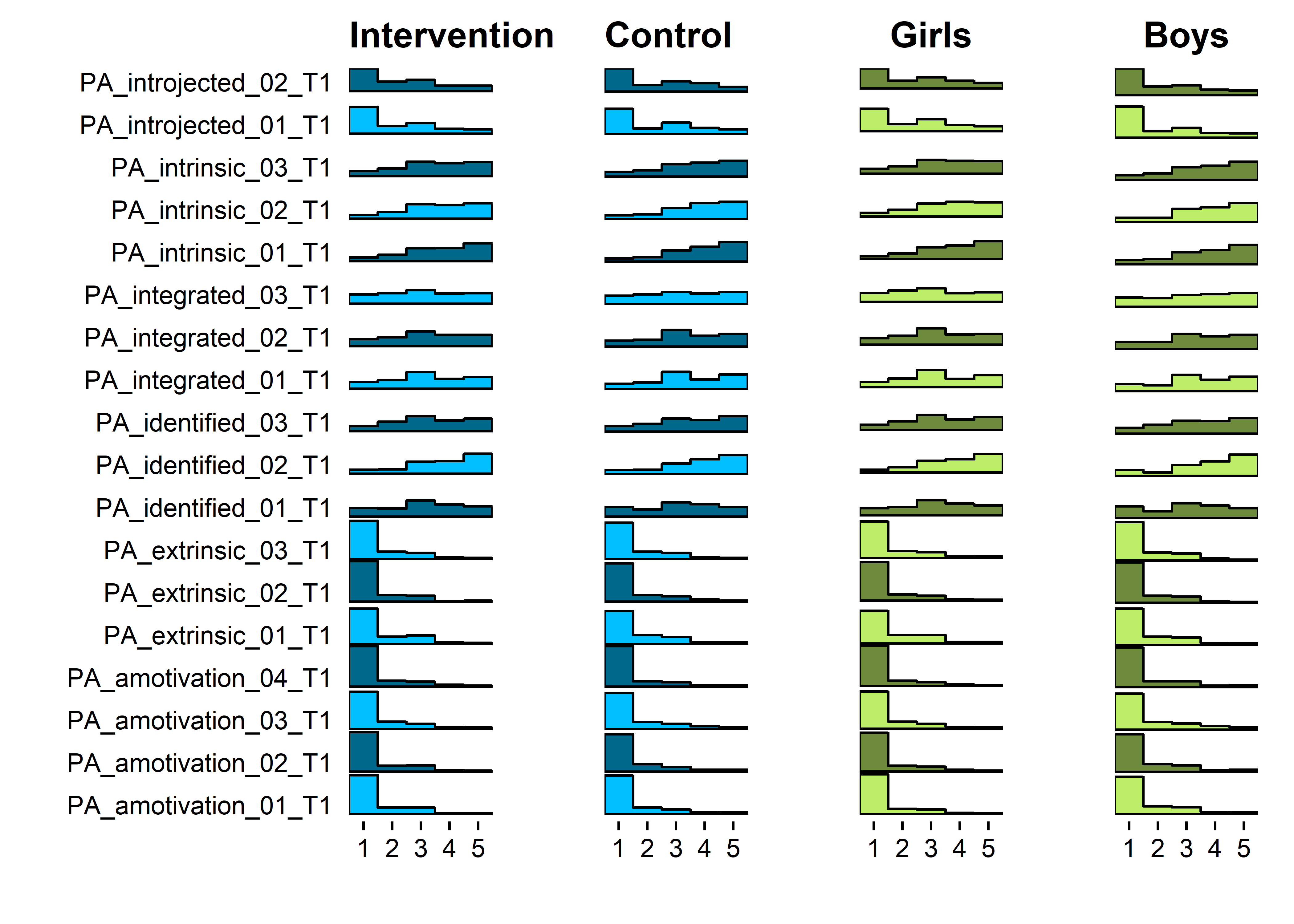
Change scores
nItems <- 18
regulations.df <- df %>% dplyr::select(
  id,
  intervention,
  group,
  school,
  girl,
  PA_amotivation_02_diff,
  PA_amotivation_01_diff,
  PA_amotivation_03_diff,
  PA_amotivation_04_diff,
  PA_extrinsic_01_diff,
  PA_extrinsic_02_diff,
  PA_extrinsic_03_diff,
  PA_introjected_01_diff,
  PA_introjected_02_diff,
  PA_identified_01_diff,
  PA_identified_02_diff,
  PA_identified_03_diff,
  PA_integrated_01_diff,
  PA_integrated_02_diff,
  PA_integrated_03_diff,
  PA_intrinsic_01_diff,
  PA_intrinsic_02_diff,
  PA_intrinsic_03_diff)


motiGirls <- regulations.df %>% dplyr::select(id,
  intervention,
  group,
  school,
  girl,
  PA_amotivation_02_diff,
  PA_amotivation_01_diff,
  PA_amotivation_03_diff,
  PA_amotivation_04_diff,
  PA_extrinsic_01_diff,
  PA_extrinsic_02_diff,
  PA_extrinsic_03_diff,
  PA_introjected_01_diff,
  PA_introjected_02_diff,
  PA_identified_01_diff,
  PA_identified_02_diff,
  PA_identified_03_diff,
  PA_integrated_01_diff,
  PA_integrated_02_diff,
  PA_integrated_03_diff,
  PA_intrinsic_01_diff,
  PA_intrinsic_02_diff,
  PA_intrinsic_03_diff) %>%
 tidyr::gather(key = Variable, value = Value, 6:ncol(.)) %>%
  filter(girl == "girl") %>%
 ggplot(aes(x = Value, y = Variable, group = Variable)) +
  ggridges::geom_density_ridges2(aes(fill = Variable), stat = "binline", binwidth = 1, scale = 0.95) +
  scale_x_continuous(breaks = c(-4:4), expand = c(0, 0),
                     name = "") +
  scale_y_discrete(expand = c(0.01, 0), name = "", labels = NULL) +
  ggridges::scale_fill_cyclical(values = c("darkolivegreen2", "darkolivegreen4")) +
  labs(title = "Girls") +
  guides(y = "none") +
  ggridges::theme_ridges(grid = FALSE) +
  theme(axis.title.x = element_text(hjust = 0.5),
        axis.title.y = element_text(hjust = 0.5),
        plot.title = element_text(hjust = 0.5),
        axis.text=element_text(size=10)) +
  coord_cartesian(xlim = c(-4, 4))
## Warning: attributes are not identical across measure variables;
## they will be dropped

motiBoys <- regulations.df %>% dplyr::select(id,
  intervention,
  group,
  school,
  girl,
  PA_amotivation_02_diff,
  PA_amotivation_01_diff,
  PA_amotivation_03_diff,
  PA_amotivation_04_diff,
  PA_extrinsic_01_diff,
  PA_extrinsic_02_diff,
  PA_extrinsic_03_diff,
  PA_introjected_01_diff,
  PA_introjected_02_diff,
  PA_identified_01_diff,
  PA_identified_02_diff,
  PA_identified_03_diff,
  PA_integrated_01_diff,
  PA_integrated_02_diff,
  PA_integrated_03_diff,
  PA_intrinsic_01_diff,
  PA_intrinsic_02_diff,
  PA_intrinsic_03_diff) %>%
 tidyr::gather(key = Variable, value = Value, 6:ncol(.)) %>%
  filter(girl == "boy") %>%
 ggplot(aes(x = Value, y = Variable, group = Variable)) +
  ggridges::geom_density_ridges2(aes(fill = Variable), stat = "binline", binwidth = 1, scale = 0.95) +
  scale_x_continuous(breaks = c(-4:4), expand = c(0, 0),
                     name = "") +
  scale_y_discrete(expand = c(0.01, 0), name = "", labels = NULL) +
  ggridges::scale_fill_cyclical(values = c("darkolivegreen2", "darkolivegreen4")) +
  labs(title = "Boys") +
  guides(y = "none") +
  ggridges::theme_ridges(grid = FALSE) +
  theme(axis.title.x = element_text(hjust = 0.5),
        axis.title.y = element_text(hjust = 0.5),
        plot.title = element_text(hjust = 0.5),
        axis.text=element_text(size=10)) +
  coord_cartesian(xlim = c(-4, 4))
## Warning: attributes are not identical across measure variables;
## they will be dropped

motiInt <- regulations.df %>% dplyr::select(id,
  intervention,
  group,
  school,
  girl,
  PA_amotivation_02_diff,
  PA_amotivation_01_diff,
  PA_amotivation_03_diff,
  PA_amotivation_04_diff,
  PA_extrinsic_01_diff,
  PA_extrinsic_02_diff,
  PA_extrinsic_03_diff,
  PA_introjected_01_diff,
  PA_introjected_02_diff,
  PA_identified_01_diff,
  PA_identified_02_diff,
  PA_identified_03_diff,
  PA_integrated_01_diff,
  PA_integrated_02_diff,
  PA_integrated_03_diff,
  PA_intrinsic_01_diff,
  PA_intrinsic_02_diff,
  PA_intrinsic_03_diff) %>%
 tidyr::gather(key = Variable, value = Value, 6:ncol(.)) %>%
  filter(intervention == "1") %>%
 ggplot(aes(x = Value, y = Variable, group = Variable)) +
  ggridges::geom_density_ridges2(aes(fill = Variable), stat = "binline", binwidth = 1, scale = 0.95) +
  scale_x_continuous(breaks = c(-4:4), expand = c(0, 0),
                     name = "") +
  scale_y_discrete(expand = c(0.01, 0), name = "") +
  ggridges::scale_fill_cyclical(values = c("deepskyblue", "deepskyblue4")) +
  labs(title = "Intervention") +
  guides(y = "none") +
  ggridges::theme_ridges(grid = FALSE) +
  theme(axis.title.x = element_text(hjust = 0.5),
        axis.title.y = element_text(hjust = 0.5),
        axis.text=element_text(size=10)) +
  coord_cartesian(xlim = c(-4, 4))
## Warning: attributes are not identical across measure variables;
## they will be dropped

motiCont <- regulations.df %>% dplyr::select(id,
  intervention,
  group,
  school,
  girl,
  PA_amotivation_02_diff,
  PA_amotivation_01_diff,
  PA_amotivation_03_diff,
  PA_amotivation_04_diff,
  PA_extrinsic_01_diff,
  PA_extrinsic_02_diff,
  PA_extrinsic_03_diff,
  PA_introjected_01_diff,
  PA_introjected_02_diff,
  PA_identified_01_diff,
  PA_identified_02_diff,
  PA_identified_03_diff,
  PA_integrated_01_diff,
  PA_integrated_02_diff,
  PA_integrated_03_diff,
  PA_intrinsic_01_diff,
  PA_intrinsic_02_diff,
  PA_intrinsic_03_diff) %>%
 tidyr::gather(key = Variable, value = Value, 6:ncol(.)) %>%
  filter(intervention == "0") %>%
 ggplot(aes(x = Value, y = Variable, group = Variable)) +
  ggridges::geom_density_ridges2(aes(fill = Variable), stat = "binline", binwidth = 1, scale = 0.95) +
  scale_x_continuous(breaks = c(-4:4), expand = c(0, 0),
                     name = "") +
  scale_y_discrete(expand = c(0.01, 0), name = "", labels = NULL) +
  ggridges::scale_fill_cyclical(values = c("deepskyblue", "deepskyblue4")) +
  labs(title = "Control") +
  guides(y = "none") +
  ggridges::theme_ridges(grid = FALSE) +
  theme(axis.title.x = element_text(hjust = 0.5),
        axis.title.y = element_text(hjust = 0.5),
        axis.text=element_text(size=10)) +
  coord_cartesian(xlim = c(-4, 4))
## Warning: attributes are not identical across measure variables;
## they will be dropped

#grid.arrange(motiInt, motiGirls, motiCont, motiBoys, ncol = 2)

# ("Seldom or never", "About once a month", "About once a week", "Almost daily")

# This draws all histograms next to each other:
grid::grid.newpage()
grid::grid.draw(cbind(ggplotGrob(motiInt), ggplotGrob(motiCont), ggplotGrob(motiGirls), ggplotGrob(motiBoys), size = "last"))
## Warning: Removed 2341 rows containing non-finite values (stat_binline).
## Warning: Removed 1804 rows containing non-finite values (stat_binline).
## Warning: Removed 2239 rows containing non-finite values (stat_binline).
## Warning: Removed 1906 rows containing non-finite values (stat_binline).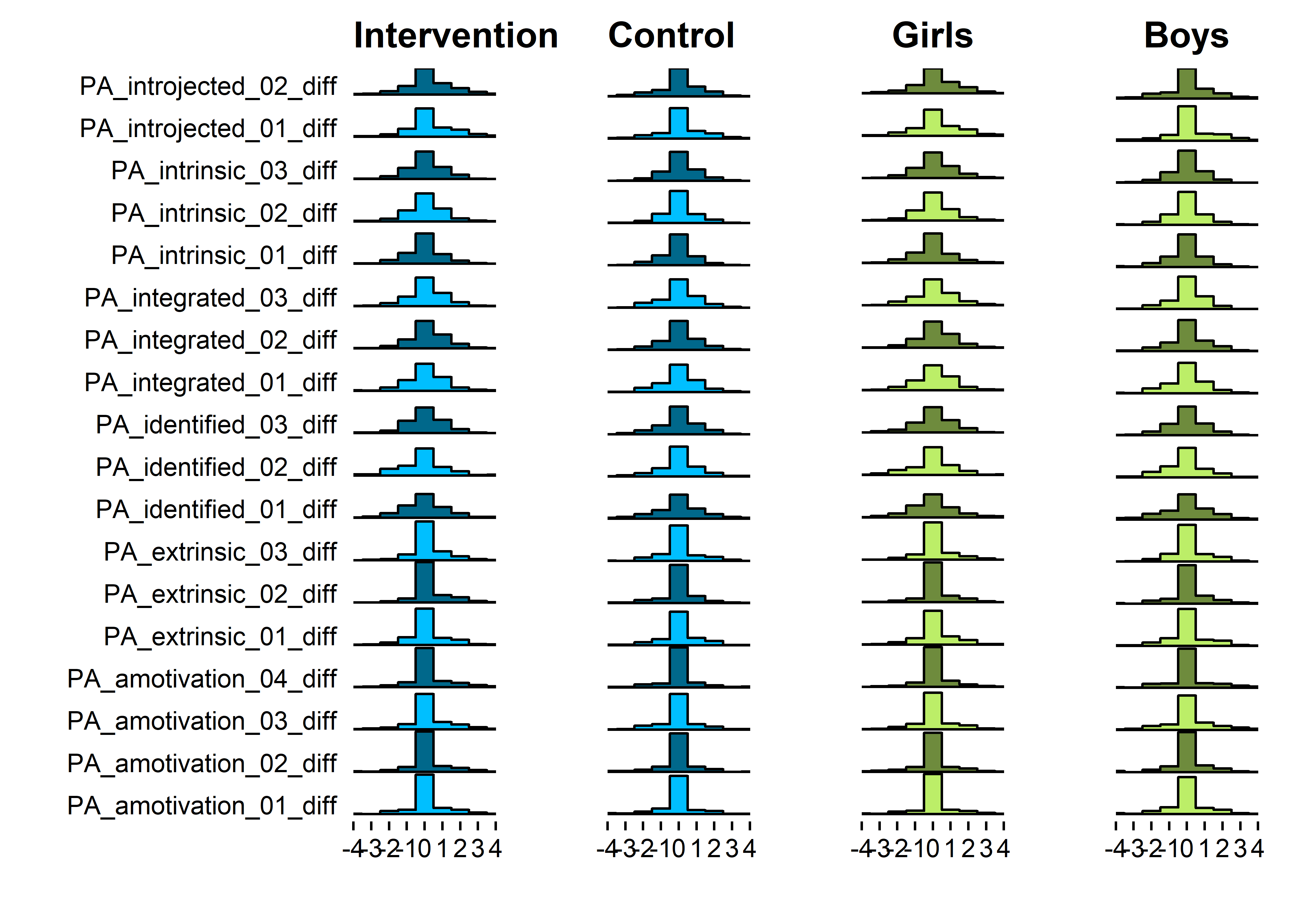
Confidence intervals
# names <- df %>% dplyr::select(-id, -intervention, -group, -school, -girl, -track, -trackSchool, -contains("_T1"), -contains("_T3")) %>% names(.)
#
# # Intercepts for boys; when boy is 1, girl is 0, but boy is a factor, so intercept is for boys even though boy is 1 for boys and 0 for girls.
# m.boys <- NA
# mean.boys <- NA
# m_p.boys <- NA
# ci_low.boys <- NA
# ci_high.boys <- NA
# ICC_group.boys <- NA
# ICC_School.boys <- NA
# nonmissings.boys <- NA
#
# df.boys <- df %>% dplyr::mutate(boy = factor(ifelse(girl == "girl", 0, 1), levels = c(1, 0)))
#
# for (i in names){
# m.boys <- lme4::lmer(paste0(i," ~ (1|school) + (1|group) + boy"), data=df.boys)
# mean.boys[i] <- lme4::fixef(m.boys)[1]
# m_p.boys <- profile(m.boys, which = "beta_")
# ci_low.boys[i] <- confint(m_p.boys)[1, 1]
# ci_high.boys[i] <- confint(m_p.boys)[1, 2]
# ICC_group.boys[i] <- sjstats::icc(m.boys)[1]
# ICC_School.boys[i] <- sjstats::icc(m.boys)[2]
# nonmissings.boys[i] <- length(m.boys@resp$y)
# }
#
# cat("The labels are arranged such that intercept is not for girls:", labels(lme4::fixef(m.boys))[2] == "boy0")
#
# ci_boys <- data.frame(ciLo = ci_low.boys, mean = mean.boys, ciHi = ci_high.boys)
# diamondlabels <- labels(ci_boys)[[1]]
# ci_boys <- data.frame(ci_boys, diamondlabels)
#
# # Intercepts for girls; when boy is 1, girl is 0, but boy is a factor, so intercept is for girls even though girl is 1 for girls and 0 for boys.
# m.girls <- NA
# mean.girls <- NA
# m_p.girls <- NA
# ci_low.girls <- NA
# ci_high.girls <- NA
# ICC_group.girls <- NA
# ICC_School.girls <- NA
# nonmissings.girls <- NA
#
# for (i in names){
# m.girls <- lme4::lmer(paste0(i," ~ (1|school) + (1|group) + girl"), data=df)
# mean.girls[i] <- lme4::fixef(m.girls)[1]
# m_p.girls <- profile(m.girls, which = "beta_")
# ci_low.girls[i] <- confint(m_p.girls)[1, 1]
# ci_high.girls[i] <- confint(m_p.girls)[1, 2]
# ICC_group.girls[i] <- sjstats::icc(m.girls)[1]
# ICC_School.girls[i] <- sjstats::icc(m.girls)[2]
# nonmissings.girls[i] <- length(m.girls@resp$y)
# }
#
# cat("The labels are arranged such that intercept is not for boys:", labels(lme4::fixef(m.girls))[2] == "girl0")
#
# ci_girls <- data.frame(ciLo = ci_low.girls, mean = mean.girls, ciHi = ci_high.girls)
# diamondlabels <- labels(ci_girls)[[1]]
# ci_girls <- data.frame(ci_girls, diamondlabels)
#
#
# # Intercepts for intervention
# m.intervention <- NA
# mean.intervention <- NA
# m_p.intervention <- NA
# ci_low.intervention <- NA
# ci_high.intervention <- NA
# ICC_group.intervention <- NA
# ICC_School.intervention <- NA
# nonmissings.intervention <- NA
#
# ## change "intervention" to be consistent regarding level order with "girl".
# df.intervention <- df %>% dplyr::mutate(intervention = factor(intervention, levels = c(1, 0)))
#
# for (i in names){
# m.intervention <- lme4::lmer(paste0(i," ~ (1|school) + (1|group) + intervention"), data=df.intervention)
# mean.intervention[i] <- lme4::fixef(m.intervention)[1]
# m_p.intervention <- profile(m.intervention, which = "beta_")
# ci_low.intervention[i] <- confint(m_p.intervention)[1, 1]
# ci_high.intervention[i] <- confint(m_p.intervention)[1, 2]
# ICC_group.intervention[i] <- sjstats::icc(m.intervention)[1]
# ICC_School.intervention[i] <- sjstats::icc(m.intervention)[2]
# nonmissings.intervention[i] <- length(m.intervention@resp$y)
# }
#
# cat("The labels are arranged such that intercept is not for control:", labels(lme4::fixef(m.intervention))[2] == "intervention0")
#
# ci_intervention <- data.frame(ciLo = ci_low.intervention, mean = mean.intervention, ciHi = ci_high.intervention)
# diamondlabels <- labels(ci_intervention)[[1]]
# ci_intervention <- data.frame(ci_intervention, diamondlabels)
#
# # Intercepts for control
#
# m.control <- NA
# mean.control <- NA
# m_p.control <- NA
# ci_low.control <- NA
# ci_high.control <- NA
# ICC_group.control <- NA
# ICC_School.control <- NA
# nonmissings.control <- NA
#
# df.control <- df %>% dplyr::mutate(control = factor(ifelse(intervention == 1, 0, 1), levels = c(1, 0)))
#
# for (i in names){
# m.control <- lme4::lmer(paste0(i," ~ (1|school) + (1|group) + control"), data=df.control)
# mean.control[i] <- lme4::fixef(m.control)[1]
# m_p.control <- profile(m.control, which = "beta_")
# ci_low.control[i] <- confint(m_p.control)[1, 1]
# ci_high.control[i] <- confint(m_p.control)[1, 2]
# ICC_group.control[i] <- sjstats::icc(m.control)[1]
# ICC_School.control[i] <- sjstats::icc(m.control)[2]
# nonmissings.control[i] <- length(m.control@resp$y)
# }
#
# cat("The labels are arranged such that intercept is not for intervention:", labels(lme4::fixef(m.control))[2] == "control0")
#
# ci_control <- data.frame(ciLo = ci_low.control, mean = mean.control, ciHi = ci_high.control)
# diamondlabels <- labels(ci_control)[[1]]
# ci_control <- data.frame(ci_control, diamondlabels)
#
# # # Same ICC results you'd get with e.g.:
# # m1 <- as.data.frame(VarCorr(m))
# # m1$vcov[1] / (m1$vcov[1] + m1$vcov[3])
#
# # Or from broom:
# # tidy(m)$estimate[2]^2 / (tidy(m)$estimate[2]^2 + tidy(m)$estimate[4]^2)
#
# # Or from sjstats:
# # sum(get_re_var(m)) / (sum(get_re_var(m)) + get_re_var(m, "sigma_2"))
#
# save(ci_control, file = "ci_control.Rdata")
# save(ci_intervention, file = "ci_intervention.Rdata")
# save(ci_girls, file = "ci_girls.Rdata")
# save(ci_boys, file = "ci_boys.Rdata")

load("ci_control.Rdata")
load("ci_intervention.Rdata")
load("ci_girls.Rdata")
load("ci_boys.Rdata")
PA determinants
plot1 <- df %>% dplyr::select(id,
  intervention,
  group,
  school,
  girl,
  padaysLastweek_T1,
'PA action and\ncoping planning' = PA_actCop_diff,
'PA intention' = PA_intention_diff,
'PA outcome\nexpectations' = PA_outcomeExpectations_diff,
'PA perceived\nbehavioural control' = PA_pbc_diff,
'PA self efficacy' = PA_selfefficacy_diff,
'PA perceived\nopportunities' = PA_opportunities_diff,
'PA descriptive\nnorm' = PA_dnorm_diff,
'PA injunctive\nnorm' = PA_inorm_diff)  %>%
  dplyr::mutate(padaysLastweek_T1 = ifelse(padaysLastweek_T1 == 0, "0",
                         ifelse(padaysLastweek_T1 == 1 | padaysLastweek_T1 == 2, "1-2",
                                ifelse(padaysLastweek_T1 >= 3, "3-7", padaysLastweek_T1)))) %>%
  dplyr::filter(!is.na(padaysLastweek_T1)) %>%
  tidyr::gather(key = Variable, value = Value, 7:(ncol(.)), factor_key = TRUE) %>%
  ggplot2::ggplot(aes(y = Variable)) +
  ggridges::geom_density_ridges(aes(x = Value,
                                    colour = "black",
                                    fill = paste(Variable, girl),
                                    point_color = girl,
                                    point_fill = girl,
                                    point_shape = girl,
                                    point_size = girl,
                                    point_alpha = girl),
                                scale = .5, alpha = .6, size = 0.25,
                                from = -6, to = 6,
                                position = position_raincloud(width = 0.03, height = 0.5),
                                jittered_points = TRUE,
                                point_size = 1) +
  scale_y_discrete(expand = c(0.01, 0)) +
  scale_x_continuous(expand = c(0.01, 0)) +
  labs(x = NULL,
       y = NULL) +
  ggridges::scale_fill_cyclical(
                      labels = c('PA action and\ncoping planning boy' = "Boy", 'PA action and\ncoping planning girl' = "Girl"),
                      values = viridis::viridis(4, end = 0.8)[c(1, 3)],
                      name = "",
                      guide = guide_legend(override.aes = list(alpha = 1,
                                                               point_shape = c(24, 25),
                                                               point_size = 2))) +
  ggridges::scale_colour_cyclical(values = "black") +
  ggridges::theme_ridges(grid = FALSE) +
  ggridges::scale_discrete_manual(aesthetics = "point_color",
                                  values = viridis::viridis(4, end = 0.8)[c(1, 3)],
                                  guide = "none") +
  ggridges::scale_discrete_manual(aesthetics = "point_fill",
                                  values = viridis::viridis(4, end = 0.8)[c(1, 3)],
                                  guide = "none") +
  ggridges::scale_discrete_manual(aesthetics = "point_shape",
                                  values = c(24, 25),
                                  guide = "none") +
  ggridges::scale_discrete_manual(aesthetics = "point_size",
                                  values = c(.75, .75),
                                  guide = "none") +
  ggridges::scale_discrete_manual(aesthetics = "point_alpha",
                                  values = c(0.1, 0.1),
                                  guide = "none") +
  papaja::theme_apa() +
  theme(legend.position = "bottom") +
  ggtitle("", subtitle = "Self-reported MVPA days, previous week") +
  facet_wrap("padaysLastweek_T1")
## Warning: attributes are not identical across measure variables;
## they will be dropped

plot1
## Picking joint bandwidth of 0.395
## Picking joint bandwidth of 0.329
## Picking joint bandwidth of 0.301
## Warning: Removed 1731 rows containing non-finite values
## (stat_density_ridges).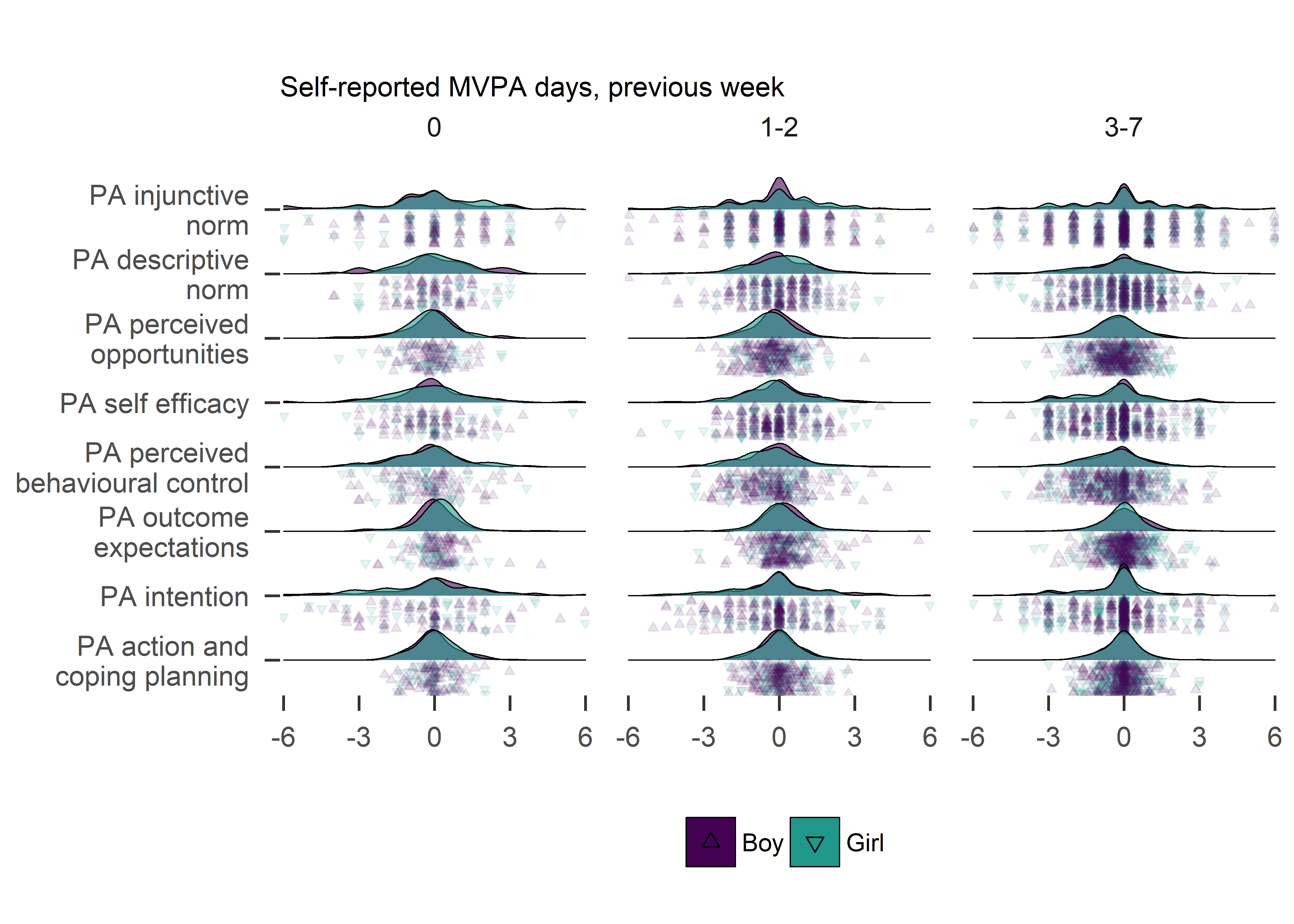
plot2 <- df %>% dplyr::select(id,
  intervention,
  group,
  school,
  girl,
  padaysLastweek_T1,
'PA action and\ncoping planning' = PA_actCop_diff,
'PA intention' = PA_intention_diff,
'PA outcome\nexpectations' = PA_outcomeExpectations_diff,
'PA perceived\nbehavioural control' = PA_pbc_diff,
'PA self efficacy' = PA_selfefficacy_diff,
'PA perceived\nopportunities' = PA_opportunities_diff,
'PA descriptive\nnorm' = PA_dnorm_diff,
'PA injunctive\nnorm' = PA_inorm_diff
)  %>%
  dplyr::mutate(padaysLastweek_T1 = ifelse(padaysLastweek_T1 == 0, "0",
                         ifelse(padaysLastweek_T1 == 1 | padaysLastweek_T1 == 2, "1-2",
                                ifelse(padaysLastweek_T1 >= 3, "3-7", padaysLastweek_T1)))) %>%
  dplyr::filter(!is.na(padaysLastweek_T1)) %>%
  tidyr::gather(key = Variable, value = Value, 7:(ncol(.)), factor_key = TRUE) %>%
  ggplot2::ggplot(aes(y = Variable)) +
  ggridges::geom_density_ridges(aes(x = Value,
                                    colour = "black",
                                    fill = paste(Variable, intervention),
                                    point_color = intervention,
                                    point_fill = intervention,
                                    point_shape = intervention,
                                    point_size = intervention,
                                    point_alpha = intervention),
                                scale = .9, alpha = .6, size = 0.25,
                                from = -6, to = 6,
                                position = position_raincloud(width = 0.03, height = 0.5),
                                jittered_points = TRUE,
                                point_size = 1) +
  scale_y_discrete(expand = c(0.01, 0)) +
  scale_x_continuous(expand = c(0.01, 0)) +
  labs(x = NULL,
       y = NULL) +
  ggridges::scale_fill_cyclical(
                      labels = c('PA action and\ncoping planning 0' = "Control", 'PA action and\ncoping planning 1' = "intervention"),
                      values = viridis::viridis(4, end = 0.8)[c(2, 4)],
                      name = "",
                      guide = guide_legend(override.aes = list(alpha = 1,
                                                               point_shape = c(21, 22),
                                                               point_size = 2))) +
  ggridges::scale_colour_cyclical(values = "black") +
  ggridges::theme_ridges(grid = FALSE) +
  ggridges::scale_discrete_manual(aesthetics = "point_color",
                                  values = viridis::viridis(4, end = 0.8)[c(2, 4)],
                                  guide = "none") +
  ggridges::scale_discrete_manual(aesthetics = "point_fill",
                                  values = viridis::viridis(4, end = 0.8)[c(2, 4)],
                                  guide = "none") +
  ggridges::scale_discrete_manual(aesthetics = "point_shape",
                                  values = c(21, 22),
                                  guide = "none") +
  ggridges::scale_discrete_manual(aesthetics = "point_size",
                                  values = c(.75, .75),
                                  guide = "none") +
  ggridges::scale_discrete_manual(aesthetics = "point_alpha",
                                  values = c(0.1, 0.1),
                                  guide = "none") +
  papaja::theme_apa() +
  theme(legend.position = "bottom") +
  ggtitle("", subtitle = "Self-reported MVPA days, previous week") +
  facet_wrap("padaysLastweek_T1")
## Warning: attributes are not identical across measure variables;
## they will be dropped

plot2
## Picking joint bandwidth of 0.413
## Picking joint bandwidth of 0.337
## Picking joint bandwidth of 0.305
## Warning: Removed 1731 rows containing non-finite values
## (stat_density_ridges).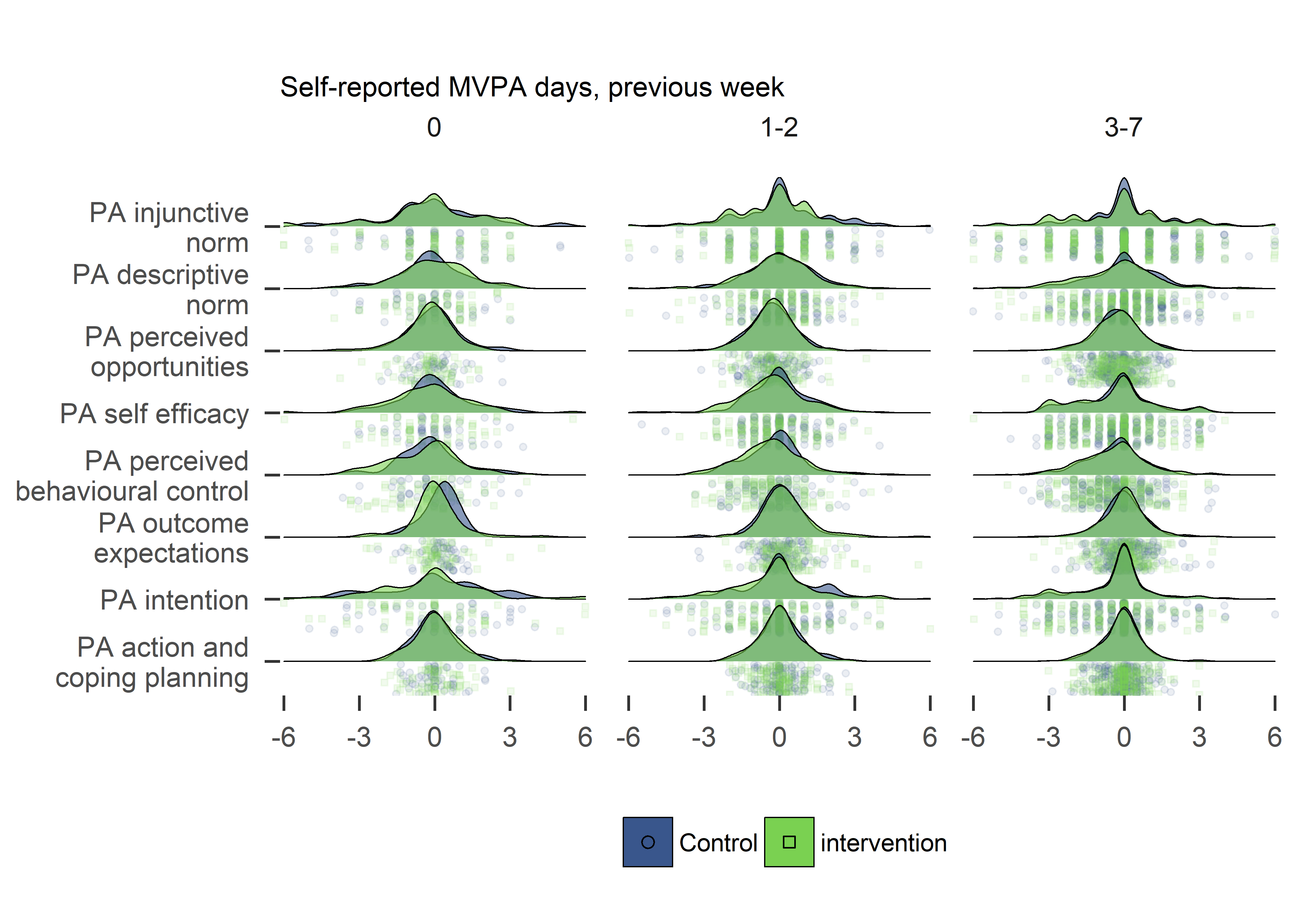
Variance in changes of determinants seems different for baseline activity.
Variance in changes by group
determinants_df <- df %>% dplyr::select(id,
  intervention,
  group,
  school,
  girl,
  padaysLastweek_T1,
'PA action and\ncoping planning' = PA_actCop_diff,
'PA intention' = PA_intention_diff,
'PA outcome\nexpectations' = PA_outcomeExpectations_diff,
'PA perceived\nbehavioural control' = PA_pbc_diff,
'PA self efficacy' = PA_selfefficacy_diff,
'PA perceived\nopportunities' = PA_opportunities_diff,
'PA descriptive\nnorm' = PA_dnorm_diff,
'PA injunctive\nnorm' = PA_inorm_diff)  %>%
  dplyr::mutate(padaysLastweek_T1 = ifelse(padaysLastweek_T1 == 0, "0",
                         ifelse(padaysLastweek_T1 == 1 | padaysLastweek_T1 == 2, "1-2",
                                ifelse(padaysLastweek_T1 >= 3, "3-7", padaysLastweek_T1)))) %>%
  dplyr::mutate_at(vars(contains("PA ")), funs(abs_dev = abs(mean(., na.rm = TRUE) - .)))


determinants_df %>% dplyr::group_by(padaysLastweek_T1, intervention) %>%
  dplyr::select(noquote(order(colnames(.)))) %>% # Orders columns alphabetically
  dplyr::summarise_at(vars(contains("PA ")), mean, na.rm = TRUE)
determinants_df %>% dplyr::group_by(padaysLastweek_T1, intervention) %>%
dplyr::select(noquote(order(colnames(.)))) %>% # Orders columns alphabetically
dplyr::summarise_at(vars(contains("PA ")), sd, na.rm = TRUE)determinants_df %>% dplyr::group_by(padaysLastweek_T1, intervention) %>%
dplyr::select(noquote(order(colnames(.)))) %>% # Orders columns alphabetically
dplyr::summarise(n = n())T2 networks compared
All regulations network
nItems <- 18
regulations.df <- df %>% dplyr::select(
  id,
  intervention,
  group,
  school,
  girl,
  PA_amotivation_02_T3,
  PA_amotivation_01_T3,
  PA_amotivation_03_T3,
  PA_amotivation_04_T3,
  PA_extrinsic_01_T3,
  PA_extrinsic_02_T3,
  PA_extrinsic_03_T3,
  PA_introjected_01_T3,
  PA_introjected_02_T3,
  PA_identified_01_T3,
  PA_identified_02_T3,
  PA_identified_03_T3,
  PA_integrated_01_T3,
  PA_integrated_02_T3,
  PA_integrated_03_T3,
  PA_intrinsic_01_T3,
  PA_intrinsic_02_T3,
  PA_intrinsic_03_T3)

regulations.df <- regulations.df %>% mutate(
PA_amotivation_02_T3 = ifelse(PA_amotivation_02_T3 == 1, 0, 1),
PA_amotivation_01_T3 = ifelse(PA_amotivation_01_T3 == 1, 0, 1),
PA_amotivation_03_T3 = ifelse(PA_amotivation_03_T3 == 1, 0, 1),
PA_amotivation_04_T3 = ifelse(PA_amotivation_04_T3 == 1, 0, 1),
PA_extrinsic_01_T3 = ifelse(PA_extrinsic_01_T3 == 1, 0, 1),
PA_extrinsic_02_T3 = ifelse(PA_extrinsic_02_T3 == 1, 0, 1),
PA_extrinsic_03_T3 = ifelse(PA_extrinsic_03_T3 == 1, 0, 1),
PA_introjected_01_T3 = ifelse(PA_introjected_01_T3 == 1, 0, 1),
PA_introjected_02_T3 = ifelse(PA_introjected_02_T3 == 1, 0, 1),
PA_identified_01_T3 = ifelse(PA_identified_01_T3 == 1, 0, 1),
PA_identified_02_T3 = ifelse(PA_identified_02_T3 == 1, 0, 1),
PA_identified_03_T3 = ifelse(PA_identified_03_T3 == 1, 0, 1),
PA_integrated_01_T3 = ifelse(PA_integrated_01_T3 == 1, 0, 1),
PA_integrated_02_T3 = ifelse(PA_integrated_02_T3 == 1, 0, 1),
PA_integrated_03_T3 = ifelse(PA_integrated_03_T3 == 1, 0, 1),
PA_intrinsic_01_T3 = ifelse(PA_intrinsic_01_T3 == 1, 0, 1),
PA_intrinsic_02_T3 = ifelse(PA_intrinsic_02_T3 == 1, 0, 1),
PA_intrinsic_03_T3 = ifelse(PA_intrinsic_03_T3 == 1, 0, 1))


### intervention AND control

S.control <- regulations.df %>% filter(intervention == "0") %>% dplyr::select(6:ncol(regulations.df)) # %>% na.omit(.)
S.intervention <- regulations.df %>% filter(intervention == "1") %>% dplyr::select(6:ncol(regulations.df)) # %>% na.omit(.)
nwcontrol <- bootnet::estimateNetwork(S.control, default="IsingFit")
## Estimating Network. Using package::function:
##   - IsingFit::IsingFit for network computation
##     - Using glmnet::glmnet
##
  |
  |                                                                 |   0%
  |
  |====                                                             |   6%
  |
  |=======                                                          |  11%
  |
  |===========                                                      |  17%
  |
  |==============                                                   |  22%
  |
  |==================                                               |  28%
  |
  |======================                                           |  33%
  |
  |=========================                                        |  39%
  |
  |=============================                                    |  44%
  |
  |================================                                 |  50%
  |
  |====================================                             |  56%
  |
  |========================================                         |  61%
  |
  |===========================================                      |  67%
  |
  |===============================================                  |  72%
  |
  |===================================================              |  78%
  |
  |======================================================           |  83%
  |
  |==========================================================       |  89%
  |
  |=============================================================    |  94%
  |
  |=================================================================| 100%
nwintervention <- bootnet::estimateNetwork(S.intervention, default="IsingFit")
## Estimating Network. Using package::function:
##   - IsingFit::IsingFit for network computation
##     - Using glmnet::glmnet
##
  |
  |                                                                 |   0%
  |
  |====                                                             |   6%
  |
  |=======                                                          |  11%
  |
  |===========                                                      |  17%
  |
  |==============                                                   |  22%
  |
  |==================                                               |  28%
  |
  |======================                                           |  33%
  |
  |=========================                                        |  39%
  |
  |=============================                                    |  44%
  |
  |================================                                 |  50%
  |
  |====================================                             |  56%
  |
  |========================================                         |  61%
  |
  |===========================================                      |  67%
  |
  |===============================================                  |  72%
  |
  |===================================================              |  78%
  |
  |======================================================           |  83%
  |
  |==========================================================       |  89%
  |
  |=============================================================    |  94%
  |
  |=================================================================| 100%

data1 <- regulations.df %>% dplyr::select(6:ncol(regulations.df))
names(data1) <- c(paste0(rep("Amoti", 4), 1:4),
                paste0(rep("Extri", 3), 1:3),
                paste0(rep("Intro", 2), 1:2),
                paste0(rep("Ident", 3), 1:3),
                paste0(rep("Integ", 3), 1:3),
                paste0(rep("Intri", 3), 1:3))
nwAll <- bootnet::estimateNetwork(data1, default="IsingFit")
## Estimating Network. Using package::function:
##   - IsingFit::IsingFit for network computation
##     - Using glmnet::glmnet
##
  |
  |                                                                 |   0%
  |
  |====                                                             |   6%
  |
  |=======                                                          |  11%
  |
  |===========                                                      |  17%
  |
  |==============                                                   |  22%
  |
  |==================                                               |  28%
  |
  |======================                                           |  33%
  |
  |=========================                                        |  39%
  |
  |=============================                                    |  44%
  |
  |================================                                 |  50%
  |
  |====================================                             |  56%
  |
  |========================================                         |  61%
  |
  |===========================================                      |  67%
  |
  |===============================================                  |  72%
  |
  |===================================================              |  78%
  |
  |======================================================           |  83%
  |
  |==========================================================       |  89%
  |
  |=============================================================    |  94%
  |
  |=================================================================| 100%

# Create means for filling nodes
interventionmeans <- regulations.df %>% group_by(intervention) %>%
  summarise_at(vars(5:(5+nItems-1)),
  funs(mean(., na.rm = TRUE))) %>%
  filter(intervention == "1") %>%
  dplyr::select(-1)

controlmeans <- regulations.df %>% group_by(intervention) %>%
  summarise_at(vars(5:(5+nItems-1)),
  funs(mean(., na.rm = TRUE))) %>%
  filter(intervention == "0") %>%
  dplyr::select(-1)

# Find average layout for comparability and plot graphs next to each other

Layout <- qgraph::averageLayout(nwintervention, nwcontrol)


layout(t(1:2))
plot(nwintervention, layout = Layout, label.scale = FALSE, title = "intervention", label.cex = 0.75,
     pie = interventionmeans,
     color = "skyblue",
     pieBorder = 1)

plot(nwcontrol, layout = Layout, label.scale = FALSE, title = "control", label.cex = 0.75,
     pie = controlmeans,
     color = "skyblue",
     pieBorder = 1)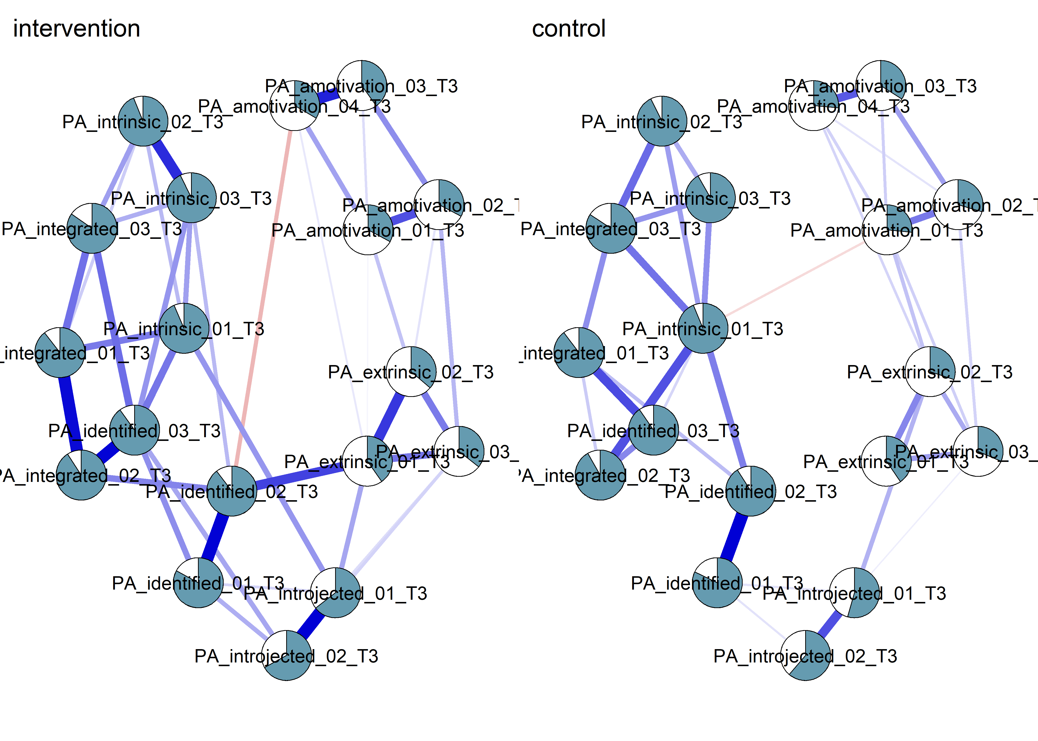
itemNames <- c('I can\'t see why I should bother exercising',
  'I do not see why I should have to exercise',
  ' I do not see the point in exercising',
  ' I think exercising is a waste of time',
  ' I exercise because other people say I should',
  ' I exercise because others will not be pleased with me if I do not',
  ' I feel under pressure from my friends/family to exercise',
  ' I feel guilty when I do not exercise',
  ' I feel like a failure when I have not exercised in a while',
  ' I think it is important to make the effort to exercise regularly',
  ' I value the benefits of exercise',
  ' it is important to me to exercise regularly',
  ' I exercise because it is consistent with my life goals.',
  ' I consider exercise consistent with my values.',
  ' I consider exercise a fundamental part of who I am.',
  ' I get pleasure and satisfaction from participating in exercise',
  ' I exercise because it is fun',
  ' I enjoy my exercise sessions')

itemGroups <- c(rep("Amotivation", 4),
                rep("Extrinsic", 3),
                rep("Introjected", 2),
                rep("Identified", 3),
                rep("Integrated", 3),
                rep("Intrinsic", 3))


plot(nwAll, groups = itemGroups, nodeNames = itemNames, legend.cex = 0.25)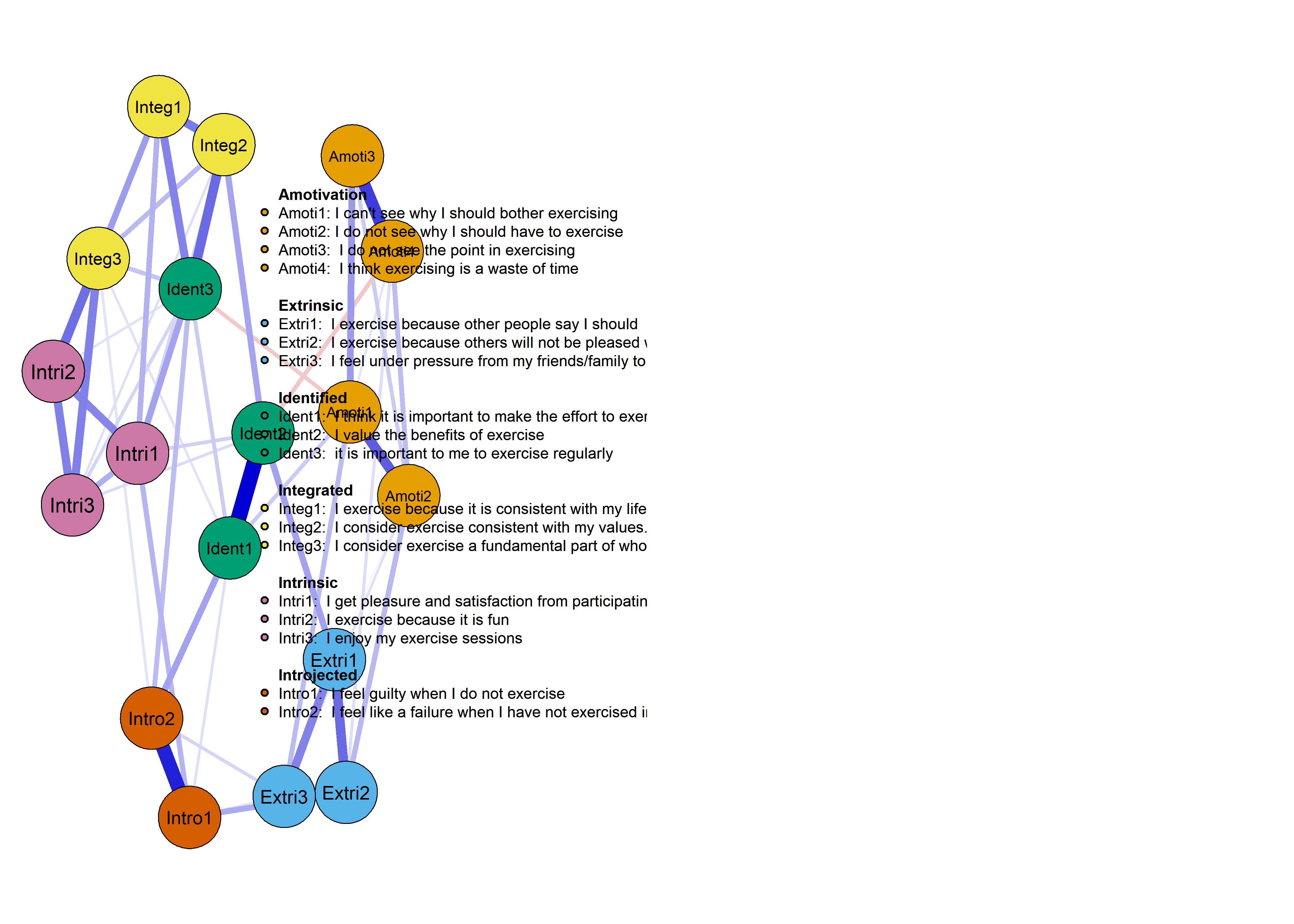
Autonomous motivation network
nItems <- 9
regulations.df <- df %>% dplyr::select(
  id,
  intervention,
  group,
  school,
  girl,
  # PA_amotivation_02_T3,
  # PA_amotivation_01_T3,
  # PA_amotivation_03_T3,
  # PA_amotivation_04_T3,
  # PA_extrinsic_01_T3,
  # PA_extrinsic_02_T3,
  # PA_extrinsic_03_T3,
  # PA_introjected_01_T3,
  # PA_introjected_02_T3,
  PA_identified_01_T3,
  PA_identified_02_T3,
  PA_identified_03_T3,
  PA_integrated_01_T3,
  PA_integrated_02_T3,
  PA_integrated_03_T3,
  PA_intrinsic_01_T3,
  PA_intrinsic_02_T3,
  PA_intrinsic_03_T3)

# regulations.df <- regulations.df %>% mutate(
# PA_amotivation_02_T3 = ifelse(PA_amotivation_02_T3 == 1, 0, 1),
# PA_amotivation_01_T3 = ifelse(PA_amotivation_01_T3 == 1, 0, 1),
# PA_amotivation_03_T3 = ifelse(PA_amotivation_03_T3 == 1, 0, 1),
# PA_amotivation_04_T3 = ifelse(PA_amotivation_04_T3 == 1, 0, 1),
# PA_extrinsic_01_T3 = ifelse(PA_extrinsic_01_T3 == 1, 0, 1),
# PA_extrinsic_02_T3 = ifelse(PA_extrinsic_02_T3 == 1, 0, 1),
# PA_extrinsic_03_T3 = ifelse(PA_extrinsic_03_T3 == 1, 0, 1),
# PA_introjected_01_T3 = ifelse(PA_introjected_01_T3 == 1, 0, 1),
# PA_introjected_02_T3 = ifelse(PA_introjected_02_T3 == 1, 0, 1),
# PA_identified_01_T3 = ifelse(PA_identified_01_T3 == 1, 0, 1),
# PA_identified_02_T3 = ifelse(PA_identified_02_T3 == 1, 0, 1),
# PA_identified_03_T3 = ifelse(PA_identified_03_T3 == 1, 0, 1),
# PA_integrated_01_T3 = ifelse(PA_integrated_01_T3 == 1, 0, 1),
# PA_integrated_02_T3 = ifelse(PA_integrated_02_T3 == 1, 0, 1),
# PA_integrated_03_T3 = ifelse(PA_integrated_03_T3 == 1, 0, 1),
# PA_intrinsic_01_T3 = ifelse(PA_intrinsic_01_T3 == 1, 0, 1),
# PA_intrinsic_02_T3 = ifelse(PA_intrinsic_02_T3 == 1, 0, 1),
# PA_intrinsic_03_T3 = ifelse(PA_intrinsic_03_T3 == 1, 0, 1))
#

### intervention and control

S.control <- regulations.df %>% filter(intervention == "0") %>%
  dplyr::select(6:ncol(regulations.df))

names(S.control) <- c(
                # paste0(rep("Amoti", 4), 1:4),
                # paste0(rep("Extri", 3), 1:3),
                # paste0(rep("Intro", 2), 1:2),
                paste0(rep("Ident", 3), 1:3),
                paste0(rep("Integ", 3), 1:3),
                paste0(rep("Intri", 3), 1:3))

S.intervention <- regulations.df %>% filter(intervention == "1") %>%
  dplyr::select(6:ncol(regulations.df))

names(S.intervention) <- c(
                # paste0(rep("Amoti", 4), 1:4),
                # paste0(rep("Extri", 3), 1:3),
                # paste0(rep("Intro", 2), 1:2),
                paste0(rep("Ident", 3), 1:3),
                paste0(rep("Integ", 3), 1:3),
                paste0(rep("Intri", 3), 1:3))

nwcontrol <- bootnet::estimateNetwork(S.control, default="EBICglasso")
## Estimating Network. Using package::function:
##   - qgraph::EBICglasso for EBIC model selection
##     - using glasso::glasso
##   - qgraph::cor_auto for correlation computation
##     - using lavaan::lavCor
## Variables detected as ordinal: Ident1; Ident2; Ident3; Integ1; Integ2; Integ3; Intri1; Intri2; Intri3
## Warning in EBICglassoCore(S = S, n = n, gamma = gamma, penalize.diagonal
## = penalize.diagonal, : A dense regularized network was selected (lambda <
## 0.1 * lambda.max). Recent work indicates a possible drop in specificity.
## Interpret the presence of the smallest edges with care. Setting threshold =
## TRUE will enforce high specificity, at the cost of sensitivity.
nwintervention <- bootnet::estimateNetwork(S.intervention, default="EBICglasso")
## Estimating Network. Using package::function:
##   - qgraph::EBICglasso for EBIC model selection
##     - using glasso::glasso
##   - qgraph::cor_auto for correlation computation
##     - using lavaan::lavCor
## Variables detected as ordinal: Ident1; Ident2; Ident3; Integ1; Integ2; Integ3; Intri1; Intri2; Intri3
## Warning in EBICglassoCore(S = S, n = n, gamma = gamma, penalize.diagonal
## = penalize.diagonal, : A dense regularized network was selected (lambda <
## 0.1 * lambda.max). Recent work indicates a possible drop in specificity.
## Interpret the presence of the smallest edges with care. Setting threshold =
## TRUE will enforce high specificity, at the cost of sensitivity.

data1 <- regulations.df %>% dplyr::select(6:ncol(regulations.df))
names(data1) <- c(
                # paste0(rep("Amoti", 4), 1:4),
                # paste0(rep("Extri", 3), 1:3),
                # paste0(rep("Intro", 2), 1:2),
                paste0(rep("Ident", 3), 1:3),
                paste0(rep("Integ", 3), 1:3),
                paste0(rep("Intri", 3), 1:3))
nwAll <- bootnet::estimateNetwork(data1, default="EBICglasso")
## Estimating Network. Using package::function:
##   - qgraph::EBICglasso for EBIC model selection
##     - using glasso::glasso
##   - qgraph::cor_auto for correlation computation
##     - using lavaan::lavCor
## Variables detected as ordinal: Ident1; Ident2; Ident3; Integ1; Integ2; Integ3; Intri1; Intri2; Intri3
## Warning in EBICglassoCore(S = S, n = n, gamma = gamma, penalize.diagonal =
## penalize.diagonal, : Network with lowest lambda selected as best network.
## Try setting 'lambda.min.ratio' lower.

## Warning in EBICglassoCore(S = S, n = n, gamma = gamma, penalize.diagonal
## = penalize.diagonal, : A dense regularized network was selected (lambda <
## 0.1 * lambda.max). Recent work indicates a possible drop in specificity.
## Interpret the presence of the smallest edges with care. Setting threshold =
## TRUE will enforce high specificity, at the cost of sensitivity.

# Create means for filling nodes
interventionmeans <- regulations.df %>% group_by(intervention) %>%
  summarise_at(vars(5:(5+nItems-1)),
  funs(mean(., na.rm = TRUE) / 5)) %>%
  filter(intervention == "1") %>%
  dplyr::select(-1)

controlmeans <- regulations.df %>% group_by(intervention) %>%
  summarise_at(vars(5:(5+nItems-1)),
  funs(mean(., na.rm = TRUE) / 5)) %>%
  filter(intervention == "0") %>%
  dplyr::select(-1)

# Find average layout for comparability and plot graphs next to each other

Layout <- qgraph::averageLayout(nwintervention, nwcontrol)

itemNames <- c(
  # 'I can\'t see why I should bother exercising',
  # 'I do not see why I should have to exercise',
  # ' I do not see the point in exercising',
  # ' I think exercising is a waste of time',
  # ' I exercise because other people say I should',
  # ' I exercise because others will not be pleased with me if I do not',
  # ' I feel under pressure from my friends/family to exercise',
  # ' I feel guilty when I do not exercise',
  # ' I feel like a failure when I have not exercised in a while',
  ' I think it is important to make the\neffort to exercise regularly',
  ' I value the benefits of exercise',
  ' it is important to me to exercise\nregularly',
  ' I exercise because it is consistent\nwith my life goals.',
  ' I consider exercise consistent with\nmy values.',
  ' I consider exercise a fundamental\npart of who I am.',
  ' I get pleasure and satisfaction from\nparticipating in exercise',
  ' I exercise because it is fun',
  ' I enjoy my exercise sessions')

itemGroups <- c(
                # rep("Amotivation", 4),
                # rep("Extrinsic", 3),
                # rep("Introjected", 2),
                rep("Identified", 3),
                rep("Integrated", 3),
                rep("Intrinsic", 3))

layout(t(1:2))
plot(nwintervention, layout = Layout, label.scale = FALSE, title = "intervention", label.cex = 0.75,
     groups = itemGroups,
     pie = interventionmeans,
     color = viridis::viridis(3, begin = 0.5, option = "B"),
     pieBorder = 1)

plot(nwcontrol, layout = Layout, label.scale = FALSE, title = "control", label.cex = 0.75,
     groups = itemGroups,
     pie = controlmeans,
     color = viridis::viridis(3, begin = 0.5, option = "B"),
     pieBorder = 1)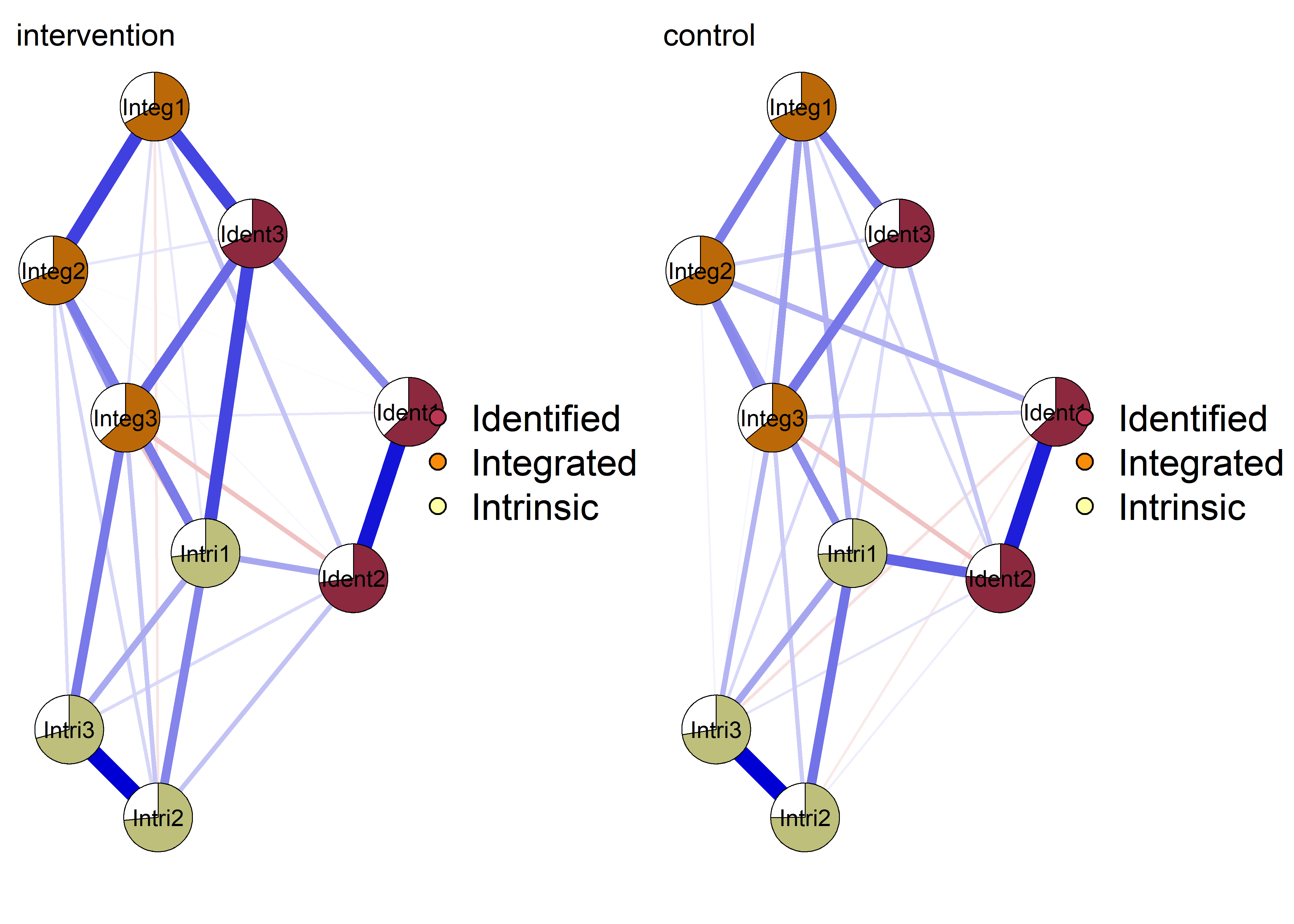
layout(1)
plot(nwAll, groups = itemGroups, nodeNames = itemNames, legend.cex = 0.4,
     color = viridis::viridis(3, begin = 0.5, option = "B"),
     mar = c(3, 10, 3, 3), layoutOffset = c(-0.75, 0))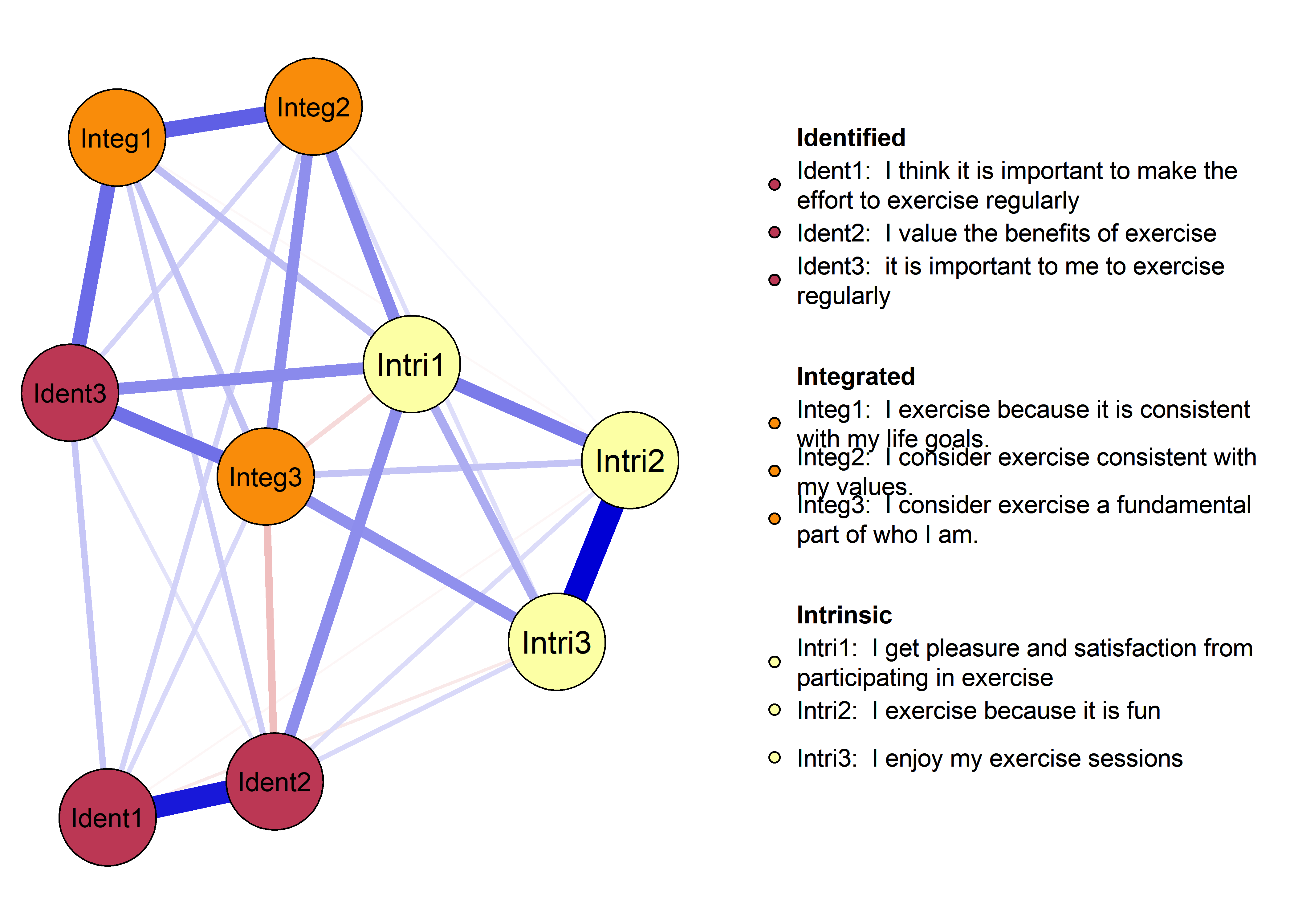
Autonomous motivation (ind. items) network with PA 1
Both accelerometer-measured MVPA (one week after filling out the survey) and self-reported PA (referring to the week prior to survey).
regulations.df <- df %>% dplyr::select(
  id,
  intervention,
  group,
  school,
  girl,
  # PA_amotivation_02_T3,
  # PA_amotivation_01_T3,
  # PA_amotivation_03_T3,
  # PA_amotivation_04_T3,
  # PA_extrinsic_01_T3,
  # PA_extrinsic_02_T3,
  # PA_extrinsic_03_T3,
  # PA_introjected_01_T3,
  # PA_introjected_02_T3,
  PA_identified_01_T3,
  PA_identified_02_T3,
  PA_identified_03_T3,
  PA_integrated_01_T3,
  PA_integrated_02_T3,
  PA_integrated_03_T3,
  PA_intrinsic_01_T3,
  PA_intrinsic_02_T3,
  PA_intrinsic_03_T3,
  padaysLastweek_T3,
  paAccelerometer_T3) %>%
  dplyr::mutate_at(vars(-(id:girl)), funs(as.numeric))

nItems <- 9

# regulations.df <- regulations.df %>% mutate(
# PA_amotivation_02_T3 = ifelse(PA_amotivation_02_T3 == 1, 0, 1),
# PA_amotivation_01_T3 = ifelse(PA_amotivation_01_T3 == 1, 0, 1),
# PA_amotivation_03_T3 = ifelse(PA_amotivation_03_T3 == 1, 0, 1),
# PA_amotivation_04_T3 = ifelse(PA_amotivation_04_T3 == 1, 0, 1),
# PA_extrinsic_01_T3 = ifelse(PA_extrinsic_01_T3 == 1, 0, 1),
# PA_extrinsic_02_T3 = ifelse(PA_extrinsic_02_T3 == 1, 0, 1),
# PA_extrinsic_03_T3 = ifelse(PA_extrinsic_03_T3 == 1, 0, 1),
# PA_introjected_01_T3 = ifelse(PA_introjected_01_T3 == 1, 0, 1),
# PA_introjected_02_T3 = ifelse(PA_introjected_02_T3 == 1, 0, 1),
# PA_identified_01_T3 = ifelse(PA_identified_01_T3 == 1, 0, 1),
# PA_identified_02_T3 = ifelse(PA_identified_02_T3 == 1, 0, 1),
# PA_identified_03_T3 = ifelse(PA_identified_03_T3 == 1, 0, 1),
# PA_integrated_01_T3 = ifelse(PA_integrated_01_T3 == 1, 0, 1),
# PA_integrated_02_T3 = ifelse(PA_integrated_02_T3 == 1, 0, 1),
# PA_integrated_03_T3 = ifelse(PA_integrated_03_T3 == 1, 0, 1),
# PA_intrinsic_01_T3 = ifelse(PA_intrinsic_01_T3 == 1, 0, 1),
# PA_intrinsic_02_T3 = ifelse(PA_intrinsic_02_T3 == 1, 0, 1),
# PA_intrinsic_03_T3 = ifelse(PA_intrinsic_03_T3 == 1, 0, 1))
#

### intervention and control

S.control <- regulations.df %>% filter(intervention == "0") %>%
  dplyr::select(6:ncol(regulations.df))

names(S.control) <- c(
                # paste0(rep("Amoti", 4), 1:4),
                # paste0(rep("Extri", 3), 1:3),
                # paste0(rep("Intro", 2), 1:2),
                paste0(rep("Ident", 3), 1:3),
                paste0(rep("Integ", 3), 1:3),
                paste0(rep("Intri", 3), 1:3),
                "Accelerom.",
                "Self-Rep.")

S.intervention <- regulations.df %>% filter(intervention == "1") %>%
  dplyr::select(6:ncol(regulations.df))

names(S.intervention) <- c(
                # paste0(rep("Amoti", 4), 1:4),
                # paste0(rep("Extri", 3), 1:3),
                # paste0(rep("Intro", 2), 1:2),
                paste0(rep("Ident", 3), 1:3),
                paste0(rep("Integ", 3), 1:3),
                paste0(rep("Intri", 3), 1:3),
                "Accelerom.",
                "Self-Rep.")

nwcontrol <- bootnet::estimateNetwork(S.control, default="EBICglasso")
## Estimating Network. Using package::function:
##   - qgraph::EBICglasso for EBIC model selection
##     - using glasso::glasso
##   - qgraph::cor_auto for correlation computation
##     - using lavaan::lavCor
## Variables detected as ordinal: Ident1; Ident2; Ident3; Integ1; Integ2; Integ3; Intri1; Intri2; Intri3
## Warning in EBICglassoCore(S = S, n = n, gamma = gamma, penalize.diagonal
## = penalize.diagonal, : A dense regularized network was selected (lambda <
## 0.1 * lambda.max). Recent work indicates a possible drop in specificity.
## Interpret the presence of the smallest edges with care. Setting threshold =
## TRUE will enforce high specificity, at the cost of sensitivity.
nwintervention <- bootnet::estimateNetwork(S.intervention, default="EBICglasso")
## Estimating Network. Using package::function:
##   - qgraph::EBICglasso for EBIC model selection
##     - using glasso::glasso
##   - qgraph::cor_auto for correlation computation
##     - using lavaan::lavCor
## Variables detected as ordinal: Ident1; Ident2; Ident3; Integ1; Integ2; Integ3; Intri1; Intri2; Intri3
## Warning in EBICglassoCore(S = S, n = n, gamma = gamma, penalize.diagonal
## = penalize.diagonal, : A dense regularized network was selected (lambda <
## 0.1 * lambda.max). Recent work indicates a possible drop in specificity.
## Interpret the presence of the smallest edges with care. Setting threshold =
## TRUE will enforce high specificity, at the cost of sensitivity.

data1 <- regulations.df %>% dplyr::select(6:ncol(regulations.df))
names(data1) <- c(
                # paste0(rep("Amoti", 4), 1:4),
                # paste0(rep("Extri", 3), 1:3),
                # paste0(rep("Intro", 2), 1:2),
                paste0(rep("Ident", 3), 1:3),
                paste0(rep("Integ", 3), 1:3),
                paste0(rep("Intri", 3), 1:3),
                "Accelerom.",
                "Self-rep.")

nwAll <- bootnet::estimateNetwork(data1, default="EBICglasso")
## Estimating Network. Using package::function:
##   - qgraph::EBICglasso for EBIC model selection
##     - using glasso::glasso
##   - qgraph::cor_auto for correlation computation
##     - using lavaan::lavCor
## Variables detected as ordinal: Ident1; Ident2; Ident3; Integ1; Integ2; Integ3; Intri1; Intri2; Intri3
## Warning in EBICglassoCore(S = S, n = n, gamma = gamma, penalize.diagonal
## = penalize.diagonal, : A dense regularized network was selected (lambda <
## 0.1 * lambda.max). Recent work indicates a possible drop in specificity.
## Interpret the presence of the smallest edges with care. Setting threshold =
## TRUE will enforce high specificity, at the cost of sensitivity.

# Create means for filling nodes
interventionmeans <- regulations.df %>%
  dplyr::group_by(intervention) %>%
  dplyr::select(-paAccelerometer_T3, -padaysLastweek_T3) %>%
  summarise_at(vars(5:(5+nItems-1)),
  funs(mean(., na.rm = TRUE) / 5)) %>%
  filter(intervention == "1") %>%
  dplyr::select(-1)

regulations.df_intervention <- regulations.df %>% filter(intervention == 1)
interventionmeans$Accelerometer <- mean(regulations.df_intervention$paAccelerometer_T3, na.rm = TRUE) / (60*24)
interventionmeans$`Self-report` <- mean(regulations.df_intervention$padaysLastweek_T3, na.rm = TRUE) / 7

controlmeans <- regulations.df %>%
  dplyr::group_by(intervention) %>%
  dplyr::select(-paAccelerometer_T3, -padaysLastweek_T3) %>%
  summarise_at(vars(5:(5+nItems-1)),
  funs(mean(., na.rm = TRUE) / 5)) %>%
  filter(intervention == "0") %>%
  dplyr::select(-1)

regulations.df_control <- regulations.df %>% filter(intervention == 0)
controlmeans$Accelerometer <- mean(regulations.df_control$paAccelerometer_T3, na.rm = TRUE) / (60*24)
controlmeans$`Self-report` <- mean(regulations.df_control$padaysLastweek_T3, na.rm = TRUE) / 7

# Find average layout for comparability and plot graphs next to each other

Layout <- qgraph::averageLayout(nwintervention, nwcontrol)

itemNames <- c(
  # 'I can\'t see why I should bother exercising',
  # 'I do not see why I should have to exercise',
  # ' I do not see the point in exercising',
  # ' I think exercising is a waste of time',
  # ' I exercise because other people say I should',
  # ' I exercise because others will not be pleased with me if I do not',
  # ' I feel under pressure from my friends/family to exercise',
  # ' I feel guilty when I do not exercise',
  # ' I feel like a failure when I have not exercised in a while',
  ' I think it is important to make the\neffort to exercise regularly',
  ' I value the benefits of exercise',
  ' it is important to me to exercise\nregularly',
  ' I exercise because it is consistent\nwith my life goals.',
  ' I consider exercise consistent with\nmy values.',
  ' I consider exercise a fundamental\npart of who I am.',
  ' I get pleasure and satisfaction from\nparticipating in exercise',
  ' I exercise because it is fun',
  ' I enjoy my exercise sessions')

itemGroups <- c(
                # rep("Amotivation", 4),
                # rep("Extrinsic", 3),
                # rep("Introjected", 2),
                rep("Identified", 3),
                rep("Integrated", 3),
                rep("Intrinsic", 3),
                "Accelerom.",
                "Self-rep.")

layout(t(1:2))
plot(nwintervention, layout = Layout, label.scale = FALSE, title = "intervention", label.cex = 0.75,
     groups = itemGroups,
     pie = interventionmeans,
     color = viridis::viridis(5, begin = 0.5, option = "B"),
     pieBorder = 1)

plot(nwcontrol, layout = Layout, label.scale = FALSE, title = "control", label.cex = 0.75,
     groups = itemGroups,
     pie = controlmeans,
     color = viridis::viridis(5, begin = 0.5, option = "B"),
     pieBorder = 1)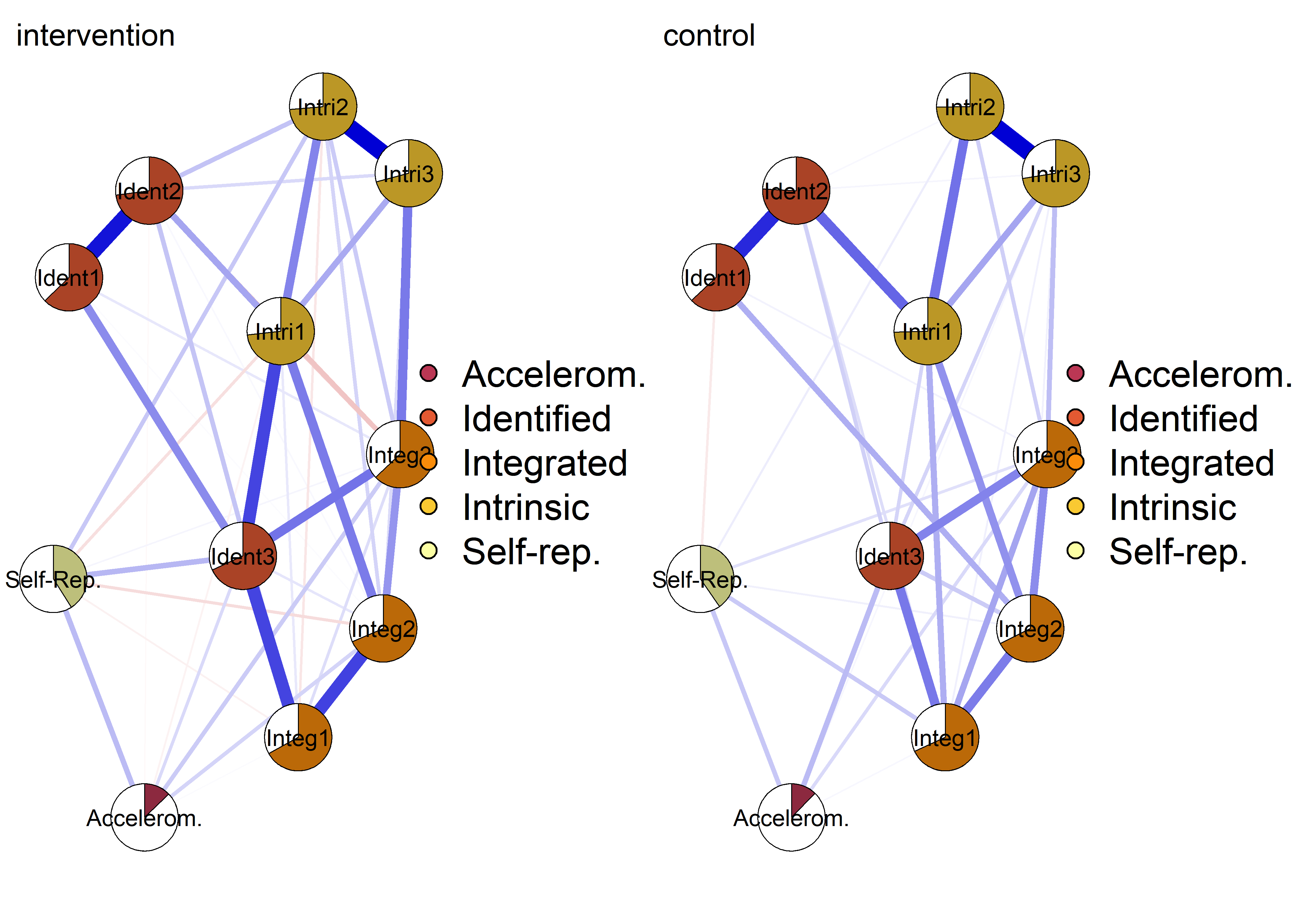
layout(1)
plot(nwAll, groups = itemGroups, nodeNames = itemNames, legend.cex = 0.4,
     color = viridis::viridis(5, begin = 0.5, option = "B"),
     mar = c(3, 10, 3, 3), layoutOffset = c(-0.75, 0))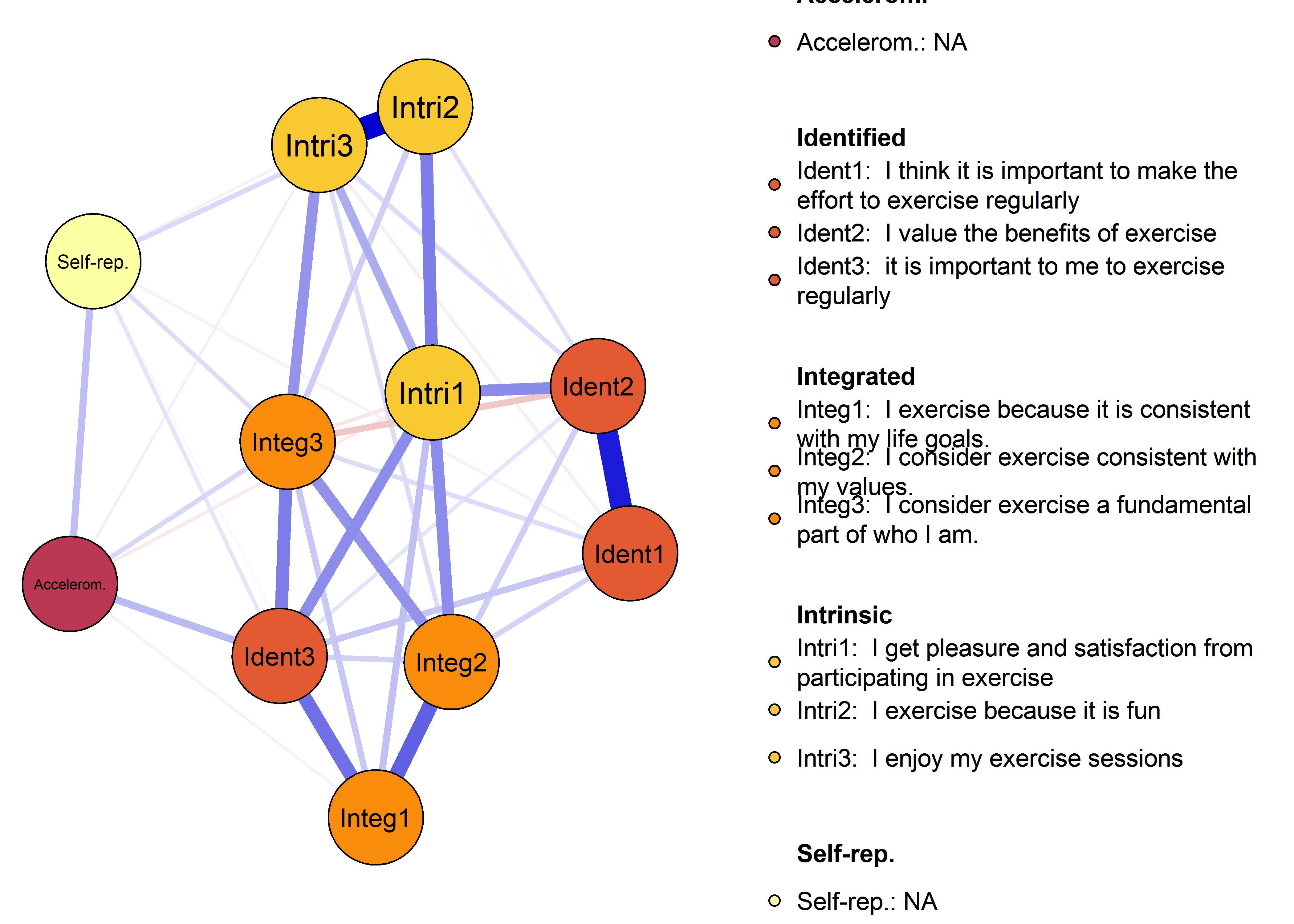
Network comparison test
# nct_results_interventionAllocation <- NetworkComparisonTest::NCT(S.control, S.intervention, it=1000, binary.data=FALSE, paired=FALSE, test.edges=TRUE,
# edges='all', progressbar=TRUE)
#
# save(nct_results_interventionAllocation, file="nct_results_interventionAllocation.Rdata")
load("nct_results_interventionAllocation.Rdata")
Print results:
print("Similarity")[1] “Similarity”
cat("Correlation between intervention and control edge strengths:", cor(qgraph::centrality(nwintervention)$InDegree, qgraph::centrality(nwcontrol)$InDegree))Correlation between intervention and control edge strengths: 0.9233915
cat("Correlation between intervention and control networks:", cor(nwintervention$graph[lower.tri(nwintervention$graph)], nwcontrol$graph[lower.tri(nwintervention$graph)], method="spearman"))Correlation between intervention and control networks: 0.6662521
print("Difference")[1] “Difference”
cat("P-value for the test of identical network structure:", nct_results_interventionAllocation$nwinv.pval)P-value for the test of identical network structure: 0.156
cat("P-value for the test of identical connectivity in networks:", nct_results_interventionAllocation$glstrinv.pval)P-value for the test of identical connectivity in networks: 0.817
nct_results_interventionAllocation$einv.pvals %>%
papaja::apa_table(caption = "p-values on difference test in edges between intervention and control group networks")| Var1 | Var2 | p-value | |
|---|---|---|---|
| 12 | Ident1 | Ident2 | 1.00 |
| 23 | Ident1 | Ident3 | 0.16 |
| 24 | Ident2 | Ident3 | 1.00 |
| 34 | Ident1 | Integ1 | 1.00 |
| 35 | Ident2 | Integ1 | 1.00 |
| 36 | Ident3 | Integ1 | 1.00 |
| 45 | Ident1 | Integ2 | 1.00 |
| 46 | Ident2 | Integ2 | 1.00 |
| 47 | Ident3 | Integ2 | 1.00 |
| 48 | Integ1 | Integ2 | 1.00 |
| 56 | Ident1 | Integ3 | 1.00 |
| 57 | Ident2 | Integ3 | 1.00 |
| 58 | Ident3 | Integ3 | 1.00 |
| 59 | Integ1 | Integ3 | 1.00 |
| 60 | Integ2 | Integ3 | 1.00 |
| 67 | Ident1 | Intri1 | 1.00 |
| 68 | Ident2 | Intri1 | 1.00 |
| 69 | Ident3 | Intri1 | 1.00 |
| 70 | Integ1 | Intri1 | 1.00 |
| 71 | Integ2 | Intri1 | 1.00 |
| 72 | Integ3 | Intri1 | 1.00 |
| 78 | Ident1 | Intri2 | 1.00 |
| 79 | Ident2 | Intri2 | 1.00 |
| 80 | Ident3 | Intri2 | 1.00 |
| 81 | Integ1 | Intri2 | 1.00 |
| 82 | Integ2 | Intri2 | 1.00 |
| 83 | Integ3 | Intri2 | 1.00 |
| 84 | Intri1 | Intri2 | 1.00 |
| 89 | Ident1 | Intri3 | 1.00 |
| 90 | Ident2 | Intri3 | 1.00 |
| 91 | Ident3 | Intri3 | 1.00 |
| 92 | Integ1 | Intri3 | 1.00 |
| 93 | Integ2 | Intri3 | 1.00 |
| 94 | Integ3 | Intri3 | 1.00 |
| 95 | Intri1 | Intri3 | 1.00 |
| 96 | Intri2 | Intri3 | 1.00 |
| 100 | Ident1 | Accelerom. | 1.00 |
| 101 | Ident2 | Accelerom. | 1.00 |
| 102 | Ident3 | Accelerom. | 1.00 |
| 103 | Integ1 | Accelerom. | 1.00 |
| 104 | Integ2 | Accelerom. | 1.00 |
| 105 | Integ3 | Accelerom. | 1.00 |
| 106 | Intri1 | Accelerom. | 1.00 |
| 107 | Intri2 | Accelerom. | 1.00 |
| 108 | Intri3 | Accelerom. | 1.00 |
| 111 | Ident1 | Self-Rep. | 1.00 |
| 112 | Ident2 | Self-Rep. | 1.00 |
| 113 | Ident3 | Self-Rep. | 1.00 |
| 114 | Integ1 | Self-Rep. | 1.00 |
| 115 | Integ2 | Self-Rep. | 1.00 |
| 116 | Integ3 | Self-Rep. | 1.00 |
| 117 | Intri1 | Self-Rep. | 1.00 |
| 118 | Intri2 | Self-Rep. | 1.00 |
| 119 | Intri3 | Self-Rep. | 1.00 |
| 120 | Accelerom. | Self-Rep. | 1.00 |
cat("Number of edges, which appear different (p<0.05):", sum(nct_results_interventionAllocation$einv.pvals$"p-value" < 0.05))Number of edges, which appear different (p<0.05): 0
Autonomous motivation (sumscores) network with PA 1
Both accelerometer-measured MVPA (one week after filling out the survey) and self-reported PA (referring to the week prior to survey).
nItems <- 3
regulations.df <- df %>% dplyr::select(
  id,
  intervention,
  group,
  school,
  girl,
  # PA_amotivation_02_T3,
  # PA_amotivation_01_T3,
  # PA_amotivation_03_T3,
  # PA_amotivation_04_T3,
  # PA_extrinsic_01_T3,
  # PA_extrinsic_02_T3,
  # PA_extrinsic_03_T3,
  # PA_introjected_01_T3,
  # PA_introjected_02_T3,
  PA_identified_T3,
  PA_integrated_T3,
  PA_intrinsic_T3,
  padaysLastweek_T3,
  paAccelerometer_T3) %>%
  dplyr::mutate_at(vars(-(id:girl)), funs(as.numeric))

# regulations.df <- regulations.df %>% mutate(
# PA_amotivation_02_T3 = ifelse(PA_amotivation_02_T3 == 1, 0, 1),
# PA_amotivation_01_T3 = ifelse(PA_amotivation_01_T3 == 1, 0, 1),
# PA_amotivation_03_T3 = ifelse(PA_amotivation_03_T3 == 1, 0, 1),
# PA_amotivation_04_T3 = ifelse(PA_amotivation_04_T3 == 1, 0, 1),
# PA_extrinsic_01_T3 = ifelse(PA_extrinsic_01_T3 == 1, 0, 1),
# PA_extrinsic_02_T3 = ifelse(PA_extrinsic_02_T3 == 1, 0, 1),
# PA_extrinsic_03_T3 = ifelse(PA_extrinsic_03_T3 == 1, 0, 1),
# PA_introjected_01_T3 = ifelse(PA_introjected_01_T3 == 1, 0, 1),
# PA_introjected_02_T3 = ifelse(PA_introjected_02_T3 == 1, 0, 1),
# PA_identified_01_T3 = ifelse(PA_identified_01_T3 == 1, 0, 1),
# PA_identified_02_T3 = ifelse(PA_identified_02_T3 == 1, 0, 1),
# PA_identified_03_T3 = ifelse(PA_identified_03_T3 == 1, 0, 1),
# PA_integrated_01_T3 = ifelse(PA_integrated_01_T3 == 1, 0, 1),
# PA_integrated_02_T3 = ifelse(PA_integrated_02_T3 == 1, 0, 1),
# PA_integrated_03_T3 = ifelse(PA_integrated_03_T3 == 1, 0, 1),
# PA_intrinsic_01_T3 = ifelse(PA_intrinsic_01_T3 == 1, 0, 1),
# PA_intrinsic_02_T3 = ifelse(PA_intrinsic_02_T3 == 1, 0, 1),
# PA_intrinsic_03_T3 = ifelse(PA_intrinsic_03_T3 == 1, 0, 1))
#

### intervention and control

S.control <- regulations.df %>% filter(intervention == "0") %>%
  dplyr::select(6:ncol(regulations.df))

names(S.control) <- c(
                # paste0(rep("Amoti", 4), 1:4),
                # paste0(rep("Extri", 1), 1),
                # paste0(rep("Intro", 2), 1:2),
                paste0(rep("Ident", 1), 1),
                paste0(rep("Integ", 1), 1),
                paste0(rep("Intri", 1), 1),
                "Accelerom.",
                "Self-Rep.")

S.intervention <- regulations.df %>% filter(intervention == "1") %>%
  dplyr::select(6:ncol(regulations.df))

names(S.intervention) <- c(
                # paste0(rep("Amoti", 4), 1:4),
                # paste0(rep("Extri", 1), 1),
                # paste0(rep("Intro", 2), 1:2),
                paste0(rep("Ident", 1), 1),
                paste0(rep("Integ", 1), 1),
                paste0(rep("Intri", 1), 1),
                "Accelerom.",
                "Self-Rep.")

nwcontrol <- bootnet::estimateNetwork(S.control, default="EBICglasso")
## Estimating Network. Using package::function:
##   - qgraph::EBICglasso for EBIC model selection
##     - using glasso::glasso
##   - qgraph::cor_auto for correlation computation
##     - using lavaan::lavCor
## Warning in EBICglassoCore(S = S, n = n, gamma = gamma, penalize.diagonal
## = penalize.diagonal, : A dense regularized network was selected (lambda <
## 0.1 * lambda.max). Recent work indicates a possible drop in specificity.
## Interpret the presence of the smallest edges with care. Setting threshold =
## TRUE will enforce high specificity, at the cost of sensitivity.
nwintervention <- bootnet::estimateNetwork(S.intervention, default="EBICglasso")
## Estimating Network. Using package::function:
##   - qgraph::EBICglasso for EBIC model selection
##     - using glasso::glasso
##   - qgraph::cor_auto for correlation computation
##     - using lavaan::lavCor
## Warning in EBICglassoCore(S = S, n = n, gamma = gamma, penalize.diagonal =
## penalize.diagonal, : Network with lowest lambda selected as best network.
## Try setting 'lambda.min.ratio' lower.

## Warning in EBICglassoCore(S = S, n = n, gamma = gamma, penalize.diagonal
## = penalize.diagonal, : A dense regularized network was selected (lambda <
## 0.1 * lambda.max). Recent work indicates a possible drop in specificity.
## Interpret the presence of the smallest edges with care. Setting threshold =
## TRUE will enforce high specificity, at the cost of sensitivity.

data1 <- regulations.df %>% dplyr::select(6:ncol(regulations.df))
names(data1) <- c(
                # paste0(rep("Amoti", 4), 1:4),
                # paste0(rep("Extri", 1), 1),
                # paste0(rep("Intro", 2), 1:2),
                paste0(rep("Ident", 1), 1),
                paste0(rep("Integ", 1), 1),
                paste0(rep("Intri", 1), 1),
                "Accelerom.",
                "Self-rep.")

nwAll <- bootnet::estimateNetwork(data1, default="EBICglasso")
## Estimating Network. Using package::function:
##   - qgraph::EBICglasso for EBIC model selection
##     - using glasso::glasso
##   - qgraph::cor_auto for correlation computation
##     - using lavaan::lavCor
## Warning in EBICglassoCore(S = S, n = n, gamma = gamma, penalize.diagonal =
## penalize.diagonal, : Network with lowest lambda selected as best network.
## Try setting 'lambda.min.ratio' lower.

## Warning in EBICglassoCore(S = S, n = n, gamma = gamma, penalize.diagonal
## = penalize.diagonal, : A dense regularized network was selected (lambda <
## 0.1 * lambda.max). Recent work indicates a possible drop in specificity.
## Interpret the presence of the smallest edges with care. Setting threshold =
## TRUE will enforce high specificity, at the cost of sensitivity.

# Create means for filling nodes
interventionmeans <- regulations.df %>%
  dplyr::group_by(intervention) %>%
  dplyr::select(-paAccelerometer_T3, -padaysLastweek_T3) %>%
  summarise_at(vars(5:(5+nItems-1)),
  funs(mean(., na.rm = TRUE) / 5)) %>%
  filter(intervention == "1") %>%
  dplyr::select(-1)

regulations.df_intervention <- regulations.df %>% filter(intervention == 1)
interventionmeans$Accelerometer <- mean(regulations.df_intervention$paAccelerometer_T3, na.rm = TRUE) / (60*24)
interventionmeans$`Self-report` <- mean(regulations.df_intervention$padaysLastweek_T3, na.rm = TRUE) / 7

controlmeans <- regulations.df %>%
  dplyr::group_by(intervention) %>%
  dplyr::select(-paAccelerometer_T3, -padaysLastweek_T3) %>%
  summarise_at(vars(5:(5+nItems-1)),
  funs(mean(., na.rm = TRUE) / 5)) %>%
  filter(intervention == "0") %>%
  dplyr::select(-1)

regulations.df_control <- regulations.df %>% filter(intervention == 0)
controlmeans$Accelerometer <- mean(regulations.df_control$paAccelerometer_T3, na.rm = TRUE) / (60*24)
controlmeans$`Self-report` <- mean(regulations.df_control$padaysLastweek_T3, na.rm = TRUE) / 7

# Find average layout for comparability and plot graphs next to each other

Layout <- qgraph::averageLayout(nwintervention, nwcontrol)

itemNames <- c(
  # 'I can\'t see why I should bother exercising',
  # 'I do not see why I should have to exercise',
  # ' I do not see the point in exercising',
  # ' I think exercising is a waste of time',
  # ' I exercise because other people say I should',
  # ' I exercise because others will not be pleased with me if I do not',
  # ' I feel under pressure from my friends/family to exercise',
  # ' I feel guilty when I do not exercise',
  # ' I feel like a failure when I have not exercised in a while',
  ' I think it is important to make the\neffort to exercise regularly',
  ' I value the benefits of exercise',
  ' it is important to me to exercise\nregularly',
  ' I exercise because it is consistent\nwith my life goals.',
  ' I consider exercise consistent with\nmy values.',
  ' I consider exercise a fundamental\npart of who I am.',
  ' I get pleasure and satisfaction from\nparticipating in exercise',
  ' I exercise because it is fun',
  ' I enjoy my exercise sessions')

itemGroups <- c(
                # rep("Amotivation", 4),
                # rep("Extrinsic", 3),
                # rep("Introjected", 2),
                rep("Identified", 1),
                rep("Integrated", 1),
                rep("Intrinsic", 1),
                "Accelerom.",
                "Self-rep.")

layout(t(1:2))
plot(nwintervention, layout = Layout, label.scale = FALSE, title = "intervention", label.cex = 0.75,
     groups = itemGroups,
     pie = interventionmeans,
     color = viridis::viridis(5, begin = 0.5, option = "B"),
     pieBorder = 1)

plot(nwcontrol, layout = Layout, label.scale = FALSE, title = "control", label.cex = 0.75,
     groups = itemGroups,
     pie = controlmeans,
     color = viridis::viridis(5, begin = 0.5, option = "B"),
     pieBorder = 1)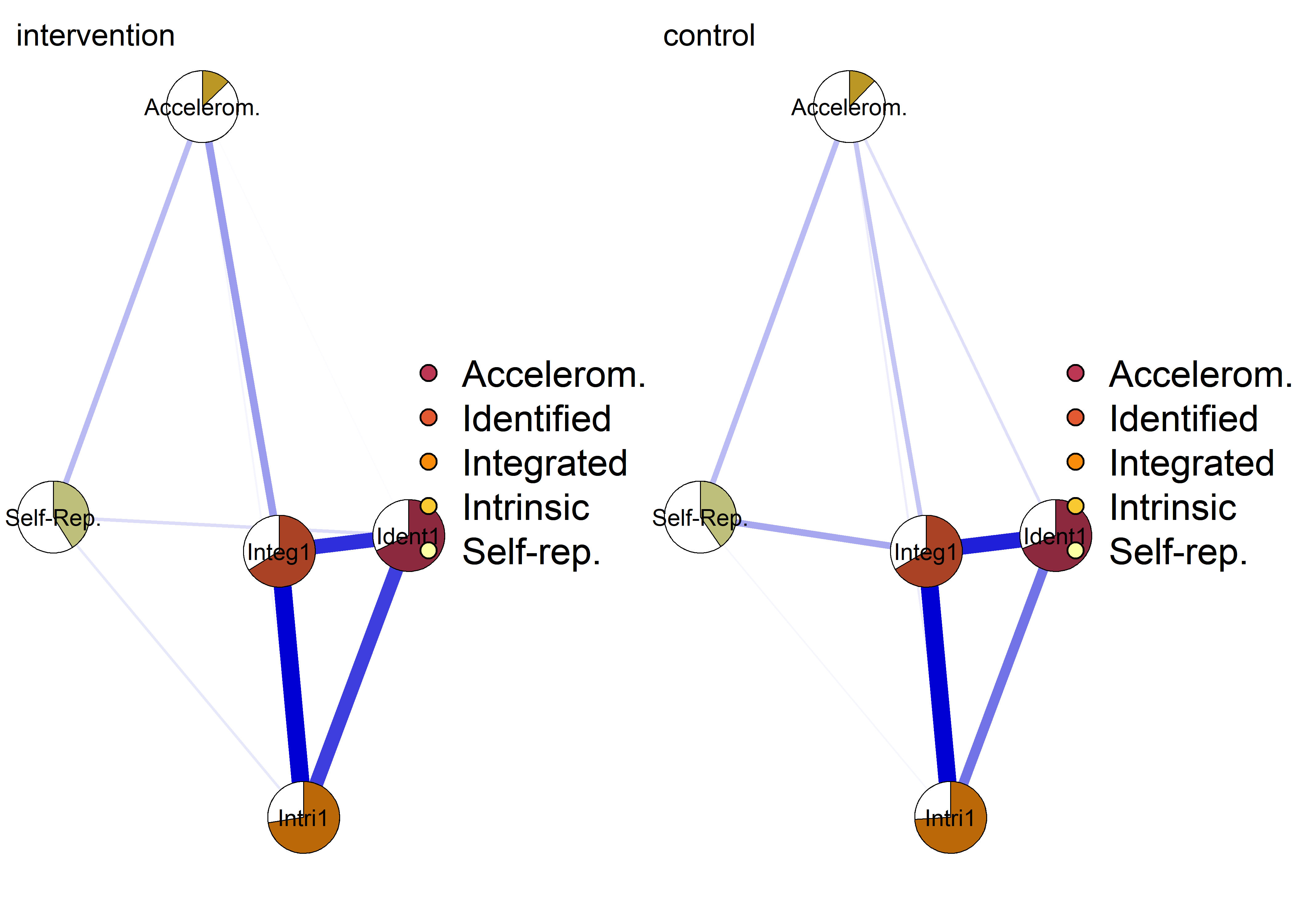
layout(1)
plot(nwAll, groups = itemGroups, nodeNames = itemNames, legend.cex = 0.4,
     color = viridis::viridis(5, begin = 0.5, option = "B"),
     mar = c(3, 10, 3, 3), layoutOffset = c(-0.75, 0))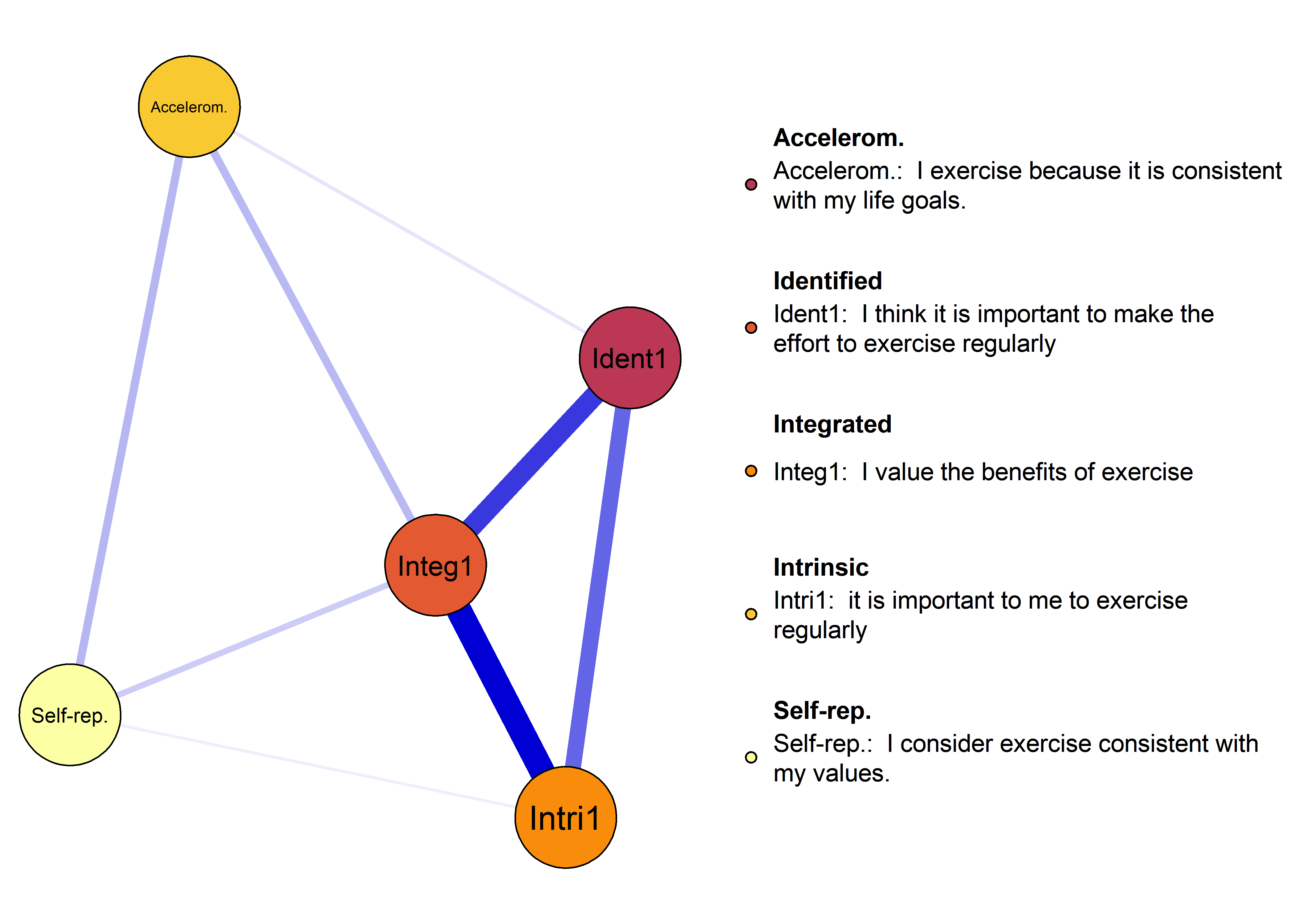
Network comparison test
# nct_results_interventionAllocation_combined_items <- NetworkComparisonTest::NCT(S.control, S.intervention, it=1000, binary.data=FALSE, paired=FALSE, test.edges=TRUE,
# edges='all', progressbar=TRUE)
#
# save(nct_results_interventionAllocation_combined_items, file="nct_results_interventionAllocation_combined_items.Rdata")
load("nct_results_interventionAllocation_combined_items.Rdata")
Print results:
print("Similarity")[1] “Similarity”
cat("Correlation between intervention and control edge strengths:", cor(qgraph::centrality(nwintervention)$InDegree, qgraph::centrality(nwcontrol)$InDegree))Correlation between intervention and control edge strengths: 0.963327
cat("Correlation between intervention and control networks:", cor(nwintervention$graph[lower.tri(nwintervention$graph)], nwcontrol$graph[lower.tri(nwintervention$graph)], method="spearman"))Correlation between intervention and control networks: 0.6121212
print("Difference")[1] “Difference”
cat("P-value for the test of identical network structure:", nct_results_interventionAllocation_combined_items$nwinv.pval)P-value for the test of identical network structure: 0.131
cat("P-value for the test of identical connectivity in networks:", nct_results_interventionAllocation_combined_items$glstrinv.pval)P-value for the test of identical connectivity in networks: 0.966
nct_results_interventionAllocation_combined_items$einv.pvals %>%
papaja::apa_table(caption = "p-values on difference test in edges between intervention and control group networks")| Var1 | Var2 | p-value | |
|---|---|---|---|
| 6 | Ident1 | Integ1 | 1.00 |
| 11 | Ident1 | Intri1 | 1.00 |
| 12 | Integ1 | Intri1 | 1.00 |
| 16 | Ident1 | Accelerom. | 1.00 |
| 17 | Integ1 | Accelerom. | 1.00 |
| 18 | Intri1 | Accelerom. | 1.00 |
| 21 | Ident1 | Self-Rep. | 1.00 |
| 22 | Integ1 | Self-Rep. | 0.10 |
| 23 | Intri1 | Self-Rep. | 1.00 |
| 24 | Accelerom. | Self-Rep. | 1.00 |
cat("Number of edges, which appear different (p<0.05):", sum(nct_results_interventionAllocation_combined_items$einv.pvals$"p-value" < 0.05))Number of edges, which appear different (p<0.05): 0