El Rogier
source("T1_plus_T3-datasetup.R")Coupling of Autonomous motivation and BCTs
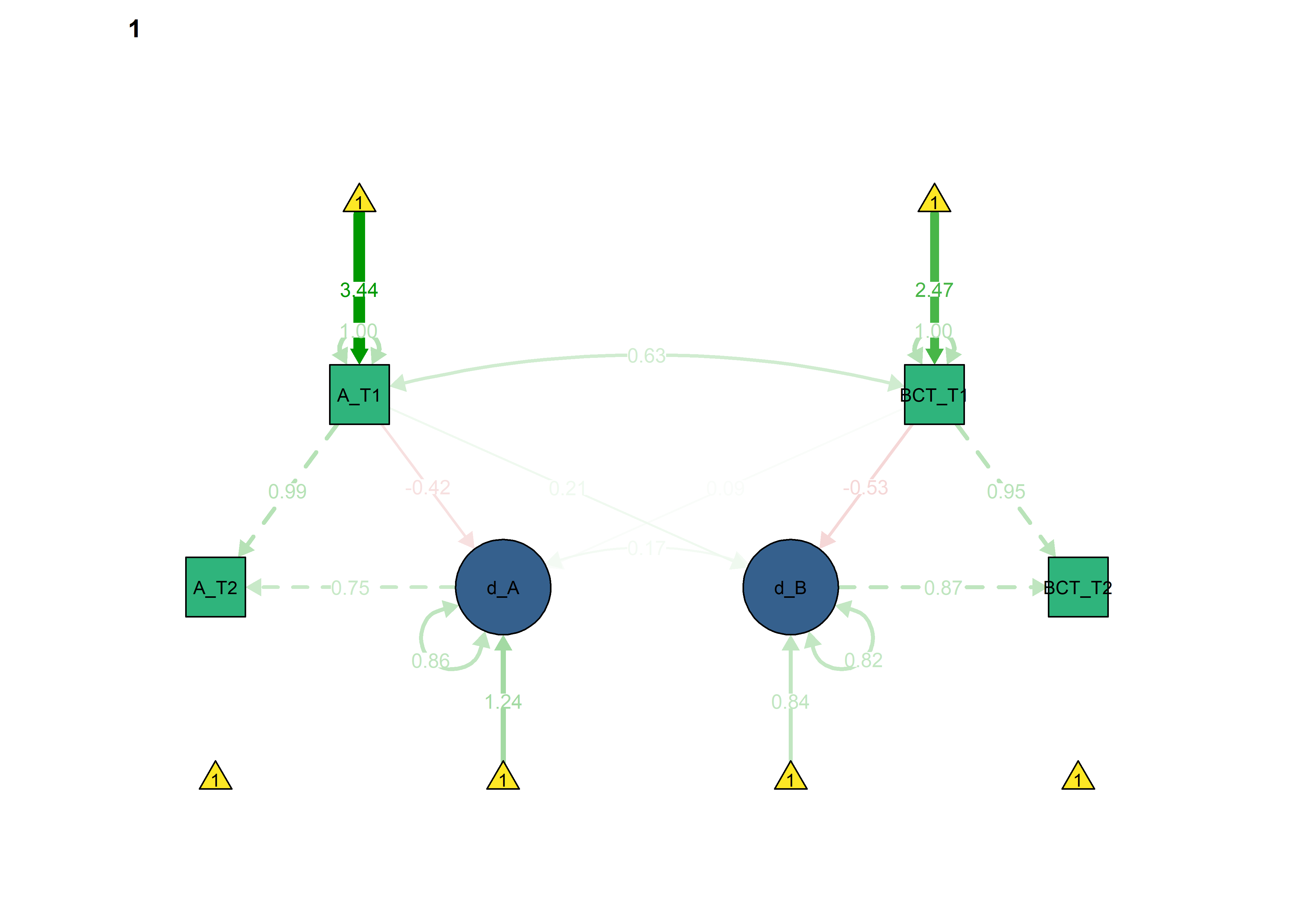
Conceptually, this model describes the mutualistic coupling of autonomous motivation to do physical activity (PA) and the use of behaviour/motivation management techniques (BCTs).
Autonomous motivation means doing things because they are pleasurable, meaningful or fitting with one’s identity.
BCTs are different techniques which help in actualising PA, as in setting goals, considering how PA fits with one’s values, etc.
The variables in this code chunk are mean scores of 9 (autonomous motivation) and 19 (BCTs) items.
Basic model
# The model in this script is originally part of the manuscript
#'Developmental cognitive neuroscience using Latent Change Score models: A tutorial and applications'
#Rogier A. Kievit, Andreas M. Brandmaier, Gabriel Ziegler, Anne-Laura van Harmelen,
#Susanne de Mooij, Michael Moutoussisa, Ian Goodyer, Ed Bullmore, Peter Jones,
#Peter Fonagy, NSPN Consortium, Ulman Lindenberger & Raymond J. Dolan
# Code was originally written by Rogier A. Kievit (rogier.kievit@mrc-cbu.cam.ac.uk), 30 January 2017.
# It may be used, (re)shared and modified freely under a CC-BY license
data_BLCS <- df %>% dplyr::select(
intervention,
Autonomous_T1 = PA_autonomous_T1,
Autonomous_T2 = PA_autonomous_T3,
frqbct_T1 = PA_frqbct_T1,
frqbct_T2 = PA_frqbct_T3,
agrbct_T1 = PA_agrbct_T1,
agrbct_T2 = PA_agrbct_T3) %>%
rowwise() %>%
dplyr::mutate(BCTs_T1 = mean(c(frqbct_T1, agrbct_T1), na.rm = TRUE),
BCTs_T2 = mean(c(frqbct_T2, agrbct_T2), na.rm = TRUE)) %>%
dplyr::select(-contains("frq"), -contains("agr"))
#Fit the Bivariate Latent Change Score model to simulated data
BLCS<-'
Autonomous_T2 ~ 1 * Autonomous_T1 # This parameter regresses Autonomous_T2 perfectly on Autonomous_T1
d_Autonomous1 =~ 1 * Autonomous_T2 # This defines the latent change score factor as measured perfectly by scores on Autonomous_T2
d_Autonomous1 ~ 1 # This estimates the intercept of the change score
Autonomous_T1 ~ 1 # This estimates the intercept of Autonomous_T1
Autonomous_T2 ~ 0 * 1 # This constrains the intercept of Autonomous_T2 to 0
BCTs_T2 ~ 1 * BCTs_T1 # This parameter regresses BCTs_T2 perfectly on BCTs_T1
d_BCTs1 =~ 1 * BCTs_T2 # This defines the latent change score factor as measured perfectly by scores on BCTs_T2
BCTs_T2 ~ 0 * 1 # This line constrains the intercept of BCTs_T2 to 0
BCTs_T2 ~~ 0 * BCTs_T2 # This fixes the variance of the BCTs_T1 to 0
d_Autonomous1 ~~ d_Autonomous1 # This estimates the variance of the change scores
Autonomous_T1 ~~ Autonomous_T1 # This estimates the variance of the Autonomous_T1
Autonomous_T2 ~~ 0 * Autonomous_T2 # This fixes the variance of the Autonomous_T2 to 0
d_BCTs1 ~ 1 # This estimates the intercept of the change score
BCTs_T1 ~ 1 # This estimates the intercept of BCTs_T1
d_BCTs1 ~~ d_BCTs1 # This estimates the variance of the change scores
BCTs_T1 ~~ BCTs_T1 # This estimates the variance of BCTs_T1
d_BCTs1 ~ Autonomous_T1 + BCTs_T1 # This estimates the autonomous to BCT coupling parameter and the BCT (T1) to BCT (T2) self-feedback
d_Autonomous1 ~ BCTs_T1 + Autonomous_T1 # This estimates the BCT to autonomous coupling parameter and the autonomous (T1) to autonomous (T2) self-feedback
Autonomous_T1 ~~ BCTs_T1 # This estimates the Autonomous_T1 BCTs_T1 covariance
d_Autonomous1 ~~ d_BCTs1 # This estimates the d_Autonomous and d_BCTs covariance
'
fitBLCS <- lavaan::lavaan(BLCS,
data = data_BLCS,
estimator = 'mlr',
fixed.x = FALSE,
group = "intervention",
missing = 'fiml')
## Warning in lav_data_full(data = data, group = group, cluster = cluster, : lavaan WARNING: group variable 'intervention' contains missing values
## Warning in lav_data_full(data = data, group = group, cluster = cluster, : lavaan WARNING: some cases are empty and will be ignored:
## 86
lavaan::summary(fitBLCS, fit.measures = TRUE, standardized = TRUE, rsquare = TRUE)
## lavaan (0.5-23.1097) converged normally after 63 iterations
##
## Number of observations per group
## 1 581
## 0 502
##
## Number of missing patterns per group
## 1 8
## 0 7
##
## Estimator ML Robust
## Minimum Function Test Statistic 0.000 0.000
## Degrees of freedom 0 0
## Minimum Function Value 0.0000000000000
## Scaling correction factor NA
## for the Yuan-Bentler correction
##
## Chi-square for each group:
##
## 1 0.000 0.000
## 0 0.000 0.000
##
## Model test baseline model:
##
## Minimum Function Test Statistic 1778.504 1178.148
## Degrees of freedom 12 12
## P-value 0.000 0.000
##
## User model versus baseline model:
##
## Comparative Fit Index (CFI) 1.000 1.000
## Tucker-Lewis Index (TLI) 1.000 1.000
##
## Robust Comparative Fit Index (CFI) NA
## Robust Tucker-Lewis Index (TLI) NA
##
## Loglikelihood and Information Criteria:
##
## Loglikelihood user model (H0) -5053.904 -5053.904
## Loglikelihood unrestricted model (H1) -5053.904 -5053.904
##
## Number of free parameters 28 28
## Akaike (AIC) 10163.807 10163.807
## Bayesian (BIC) 10303.457 10303.457
## Sample-size adjusted Bayesian (BIC) 10214.523 10214.523
##
## Root Mean Square Error of Approximation:
##
## RMSEA 0.000 0.000
## 90 Percent Confidence Interval 0.000 0.000 0.000 0.000
## P-value RMSEA <= 0.05 NA NA
##
## Robust RMSEA 0.000
## 90 Percent Confidence Interval 0.000 0.000
##
## Standardized Root Mean Square Residual:
##
## SRMR 0.000 0.000
##
## Parameter Estimates:
##
## Information Observed
## Standard Errors Robust.huber.white
##
##
## Group 1 [1]:
##
## Latent Variables:
## Estimate Std.Err z-value P(>|z|) Std.lv Std.all
## d_Autonomous1 =~
## Autonomous_T2 1.000 0.816 0.777
## d_BCTs1 =~
## BCTs_T2 1.000 1.013 0.809
##
## Regressions:
## Estimate Std.Err z-value P(>|z|) Std.lv Std.all
## Autonomous_T2 ~
## Autonomous_T1 1.000 1.000 1.010
## BCTs_T2 ~
## BCTs_T1 1.000 1.000 0.913
## d_BCTs1 ~
## Autonomous_T1 0.229 0.058 3.933 0.000 0.226 0.240
## BCTs_T1 -0.419 0.062 -6.791 0.000 -0.414 -0.473
## d_Autonomous1 ~
## BCTs_T1 0.131 0.046 2.852 0.004 0.161 0.184
## Autonomous_T1 -0.390 0.052 -7.516 0.000 -0.478 -0.507
##
## Covariances:
## Estimate Std.Err z-value P(>|z|) Std.lv Std.all
## Autonomous_T1 ~~
## BCTs_T1 0.725 0.052 14.025 0.000 0.725 0.598
## .d_Autonomous1 ~~
## .d_BCTs1 0.202 0.041 4.894 0.000 0.291 0.291
##
## Intercepts:
## Estimate Std.Err z-value P(>|z|) Std.lv Std.all
## .d_Autonomous1 1.003 0.129 7.797 0.000 1.228 1.228
## Autonomous_T1 3.355 0.044 76.132 0.000 3.355 3.161
## .Autonomous_T2 0.000 0.000 0.000
## .BCTs_T2 0.000 0.000 0.000
## .d_BCTs1 0.626 0.132 4.730 0.000 0.618 0.618
## BCTs_T1 2.768 0.048 58.203 0.000 2.768 2.421
##
## Variances:
## Estimate Std.Err z-value P(>|z|) Std.lv Std.all
## .BCTs_T2 0.000 0.000 0.000
## .d_Autonomous1 0.547 0.051 10.768 0.000 0.821 0.821
## Autonomous_T1 1.126 0.053 21.199 0.000 1.126 1.000
## .Autonomous_T2 0.000 0.000 0.000
## .d_BCTs1 0.877 0.062 14.158 0.000 0.854 0.854
## BCTs_T1 1.308 0.073 17.859 0.000 1.308 1.000
##
## R-Square:
## Estimate
## BCTs_T2 1.000
## d_Autonomous1 0.179
## Autonomous_T2 1.000
## d_BCTs1 0.146
##
##
## Group 2 [0]:
##
## Latent Variables:
## Estimate Std.Err z-value P(>|z|) Std.lv Std.all
## d_Autonomous1 =~
## Autonomous_T2 1.000 0.671 0.650
## d_BCTs1 =~
## BCTs_T2 1.000 1.032 0.875
##
## Regressions:
## Estimate Std.Err z-value P(>|z|) Std.lv Std.all
## Autonomous_T2 ~
## Autonomous_T1 1.000 1.000 1.006
## BCTs_T2 ~
## BCTs_T1 1.000 1.000 0.981
## d_BCTs1 ~
## Autonomous_T1 0.255 0.061 4.177 0.000 0.247 0.257
## BCTs_T1 -0.523 0.059 -8.860 0.000 -0.507 -0.586
## d_Autonomous1 ~
## BCTs_T1 0.112 0.043 2.626 0.009 0.167 0.193
## Autonomous_T1 -0.293 0.044 -6.582 0.000 -0.437 -0.453
##
## Covariances:
## Estimate Std.Err z-value P(>|z|) Std.lv Std.all
## Autonomous_T1 ~~
## BCTs_T1 0.758 0.054 14.090 0.000 0.758 0.631
## .d_Autonomous1 ~~
## .d_BCTs1 0.100 0.032 3.119 0.002 0.175 0.175
##
## Intercepts:
## Estimate Std.Err z-value P(>|z|) Std.lv Std.all
## .d_Autonomous1 0.729 0.103 7.067 0.000 1.086 1.086
## Autonomous_T1 3.475 0.046 74.929 0.000 3.475 3.347
## .Autonomous_T2 0.000 0.000 0.000
## .BCTs_T2 0.000 0.000 0.000
## .d_BCTs1 0.637 0.142 4.476 0.000 0.617 0.617
## BCTs_T1 2.876 0.052 55.593 0.000 2.876 2.489
##
## Variances:
## Estimate Std.Err z-value P(>|z|) Std.lv Std.all
## .BCTs_T2 0.000 0.000 0.000
## .d_Autonomous1 0.390 0.032 12.254 0.000 0.868 0.868
## Autonomous_T1 1.078 0.058 18.469 0.000 1.078 1.000
## .Autonomous_T2 0.000 0.000 0.000
## .d_BCTs1 0.830 0.064 13.046 0.000 0.781 0.781
## BCTs_T1 1.336 0.067 19.898 0.000 1.336 1.000
##
## R-Square:
## Estimate
## BCTs_T2 1.000
## d_Autonomous1 0.132
## Autonomous_T2 1.000
## d_BCTs1 0.219
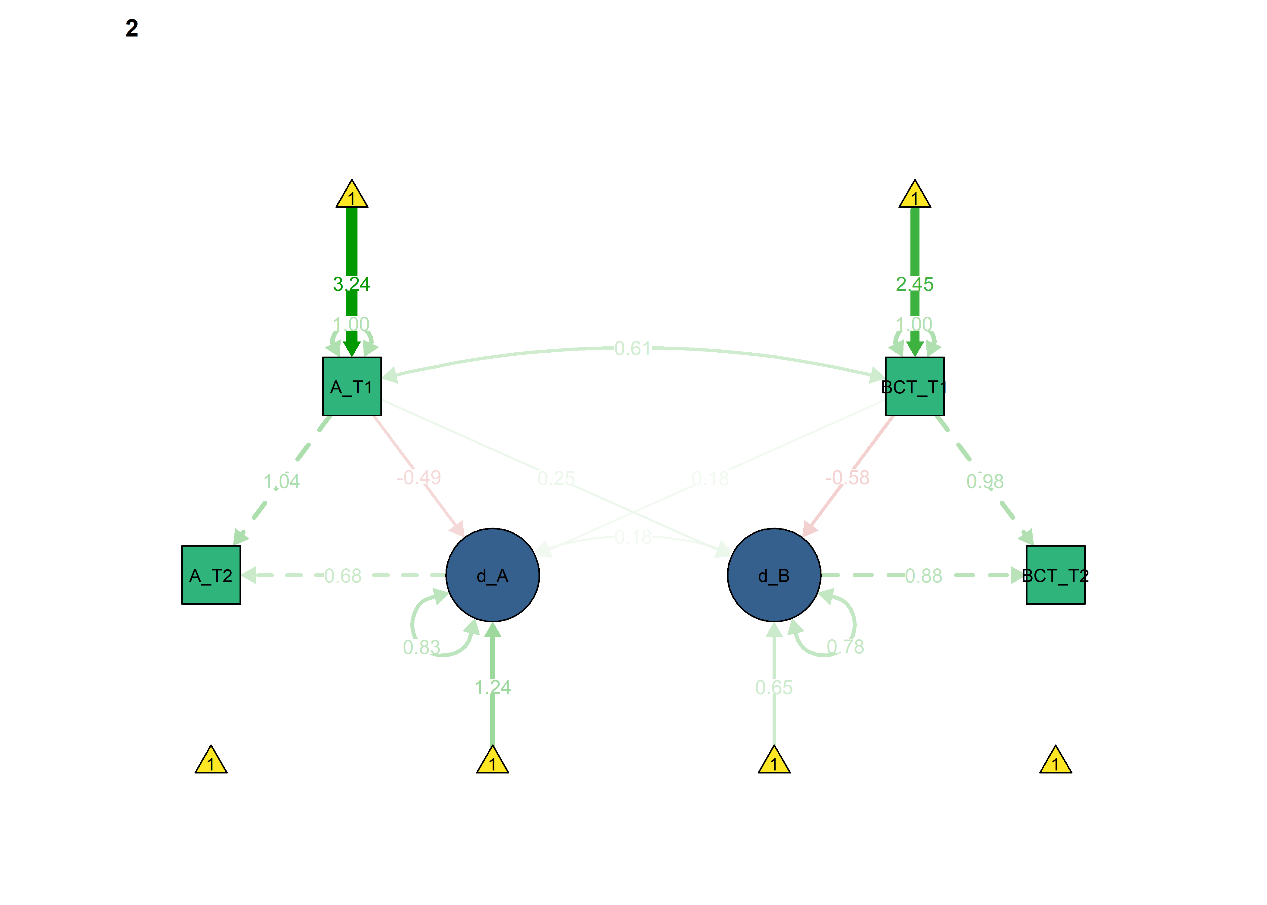
semPlot::semPaths(fitBLCS,
what = "std",
ask = FALSE,
label.cex = .6,
label.scale = FALSE,
edge.label.cex = 0.75,
layout = "tree2",
intercepts = TRUE,
color = list(lat = viridis::viridis(3, begin = 0.3)[1],
man = viridis::viridis(3, begin = 0.3)[2],
int = viridis::viridis(3, begin = 0.3)[3]))

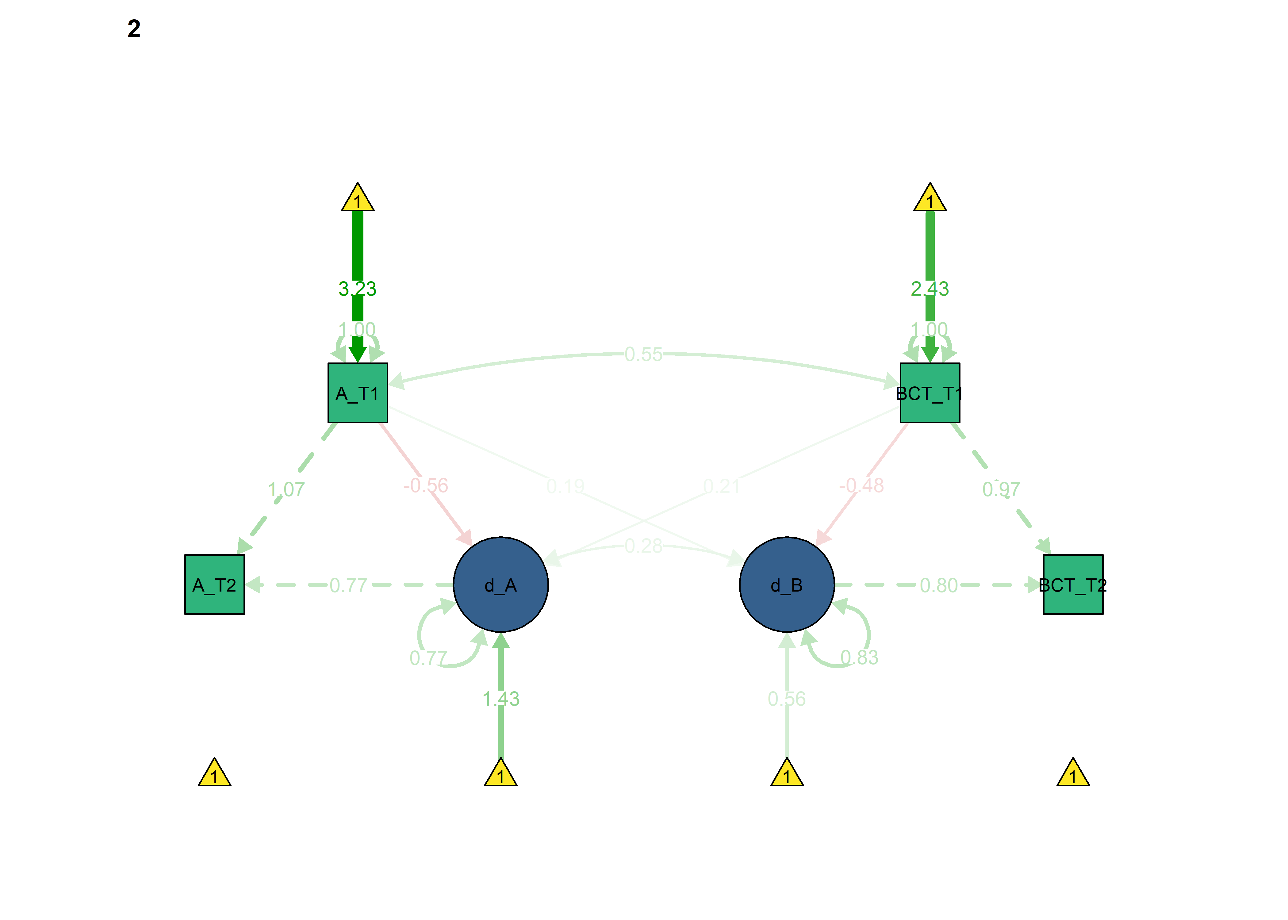
Constrained model
Next, we constrain parameters, which ought to be the same across groups, as identical:
- the intercept of Autonomous_T1
- the variance of the Autonomous_T1
- the intercept of BCTs_T1
- the variance of BCTs_T1
- the covariance between Autonomous_T1 and BCTs_T1
data_BLCS <- df %>% dplyr::select(
  intervention,
  Autonomous_T1 = PA_autonomous_T1,
  Autonomous_T2 = PA_autonomous_T3,
  frqbct_T1 = PA_frqbct_T1,
  frqbct_T2 = PA_frqbct_T3,
  agrbct_T1 = PA_agrbct_T1,
  agrbct_T2 = PA_agrbct_T3) %>%
  rowwise() %>%
  dplyr::mutate(BCTs_T1 = mean(c(frqbct_T1, agrbct_T1), na.rm = TRUE),
                BCTs_T2 = mean(c(frqbct_T2, agrbct_T2), na.rm = TRUE)) %>%
  dplyr::select(-contains("frq"), -contains("agr"))


#Fit the Bivariate Latent Change Score model to simulated data
BLCS_constrained <- '

Autonomous_T2 ~ 1 * Autonomous_T1     # This parameter regresses Autonomous_T2 perfectly on Autonomous_T1
d_Autonomous1 =~ 1 * Autonomous_T2    # This defines the latent change score factor as measured perfectly by scores on Autonomous_T2
d_Autonomous1 ~ 1                     # This estimates the intercept of the change score
Autonomous_T1 ~  c(autint, autint)*1  # This constrains the intercept of Autonomous_T1 to be identical across intervention and control groups
Autonomous_T2 ~ 0 * 1                 # This constrains the intercept of Autonomous_T2 to 0

BCTs_T2 ~ 1 * BCTs_T1     # This parameter regresses BCTs_T2 perfectly on BCTs_T1
d_BCTs1 =~ 1 * BCTs_T2    # This defines the latent change score factor as measured perfectly by scores on BCTs_T2
BCTs_T2 ~ 0 * 1           # This line constrains the intercept of BCTs_T2 to 0
BCTs_T2 ~~ 0 * BCTs_T2    # This fixes the variance of the BCTs_T1 to 0

d_Autonomous1 ~~  d_Autonomous1                     # This estimates the variance of the change scores
Autonomous_T1 ~~ c(autvar, autvar) * Autonomous_T1  # This estimates the variance of the Autonomous_T1
Autonomous_T2 ~~ 0 * Autonomous_T2                  # This fixes the variance of the Autonomous_T2 to 0

d_BCTs1 ~ 1                            # This estimates the intercept of the change score
BCTs_T1 ~ c(bctint, bctint) * 1        # This estimates the intercept of BCTs_T1
d_BCTs1 ~~ d_BCTs1                     # This estimates the variance of the change scores
BCTs_T1 ~~ c(bctvar, bctvar) * BCTs_T1 # This estimates the variance of BCTs_T1

d_BCTs1 ~ Autonomous_T1 + BCTs_T1       # This estimates the autonomous to BCT coupling parameter and the BCT (T1) to BCT (T2) self-feedback
d_Autonomous1 ~ BCTs_T1 + Autonomous_T1 # This estimates the BCT to autonomous coupling parameter and the autonomous (T1) to autonomous (T2) self-feedback

Autonomous_T1 ~~ c(autbct_cov, autbct_cov) * BCTs_T1                    # This estimates the Autonomous_T1 BCTs_T1 covariance
d_Autonomous1 ~~ d_BCTs1                      # This estimates the d_Autonomous and d_BCTs covariance
'

fitBLCS_constrained <- lavaan::lavaan(BLCS_constrained,
                          data = data_BLCS,
                          estimator = 'mlr',
                          fixed.x = FALSE,
                          group = "intervention",
                          missing = 'fiml')
## Warning in lav_data_full(data = data, group = group, cluster = cluster, : lavaan WARNING: group variable 'intervention' contains missing values
## Warning in lav_data_full(data = data, group = group, cluster = cluster, : lavaan WARNING: some cases are empty and will be ignored:
##   86

lavaan::summary(fitBLCS_constrained, fit.measures = TRUE, standardized = TRUE, rsquare = TRUE)
## lavaan (0.5-23.1097) converged normally after  56 iterations
##
##   Number of observations per group
##   1                                                581
##   0                                                502
##
##   Number of missing patterns per group
##   1                                                  8
##   0                                                  7
##
##   Estimator                                         ML      Robust
##   Minimum Function Test Statistic                5.540       5.945
##   Degrees of freedom                                 5           5
##   P-value (Chi-square)                           0.354       0.312
##   Scaling correction factor                                  0.932
##     for the Yuan-Bentler correction
##
## Chi-square for each group:
##
##   1                                              2.524       2.709
##   0                                              3.016       3.236
##
## Model test baseline model:
##
##   Minimum Function Test Statistic             1778.504    1178.148
##   Degrees of freedom                                12          12
##   P-value                                        0.000       0.000
##
## User model versus baseline model:
##
##   Comparative Fit Index (CFI)                    1.000       0.999
##   Tucker-Lewis Index (TLI)                       0.999       0.998
##
##   Robust Comparative Fit Index (CFI)                         0.999
##   Robust Tucker-Lewis Index (TLI)                            0.999
##
## Loglikelihood and Information Criteria:
##
##   Loglikelihood user model (H0)              -5056.674   -5056.674
##   Scaling correction factor                                  0.979
##     for the MLR correction
##   Loglikelihood unrestricted model (H1)      -5053.904   -5053.904
##   Scaling correction factor                                  1.145
##     for the MLR correction
##
##   Number of free parameters                         23          23
##   Akaike (AIC)                               10159.348   10159.348
##   Bayesian (BIC)                             10274.060   10274.060
##   Sample-size adjusted Bayesian (BIC)        10201.007   10201.007
##
## Root Mean Square Error of Approximation:
##
##   RMSEA                                          0.014       0.019
##   90 Percent Confidence Interval          0.000  0.063       0.000  0.066
##   P-value RMSEA <= 0.05                          0.859       0.824
##
##   Robust RMSEA                                               0.018
##   90 Percent Confidence Interval                             0.000  0.063
##
## Standardized Root Mean Square Residual:
##
##   SRMR                                           0.027       0.027
##
## Parameter Estimates:
##
##   Information                                 Observed
##   Standard Errors                   Robust.huber.white
##
##
## Group 1 [1]:
##
## Latent Variables:
##                    Estimate  Std.Err  z-value  P(>|z|)   Std.lv  Std.all
##   d_Autonomous1 =~
##     Autonomous_T2     1.000                               0.814    0.775
##   d_BCTs1 =~
##     BCTs_T2           1.000                               1.012    0.806
##
## Regressions:
##                    Estimate  Std.Err  z-value  P(>|z|)   Std.lv  Std.all
##   Autonomous_T2 ~
##     Autonomous_T1     1.000                               1.000    1.003
##   BCTs_T2 ~
##     BCTs_T1           1.000                               1.000    0.916
##   d_BCTs1 ~
##     Autonomous_T1     0.229    0.058    3.933    0.000    0.227    0.238
##     BCTs_T1          -0.419    0.062   -6.791    0.000   -0.414   -0.477
##   d_Autonomous1 ~
##     BCTs_T1           0.131    0.046    2.851    0.004    0.162    0.186
##     Autonomous_T1    -0.390    0.052   -7.516    0.000   -0.479   -0.504
##
## Covariances:
##                    Estimate  Std.Err  z-value  P(>|z|)   Std.lv  Std.all
##   Autonomous_T1 ~~
##     BCTs_T1 (atb_)    0.743    0.037   20.055    0.000    0.743    0.614
##  .d_Autonomous1 ~~
##    .d_BCTs1           0.202    0.041    4.894    0.000    0.291    0.291
##
## Intercepts:
##                    Estimate  Std.Err  z-value  P(>|z|)   Std.lv  Std.all
##    .d_Atnm1           1.003    0.129    7.796    0.000    1.232    1.232
##     Atnm_T1 (atnt)    3.411    0.032  106.563    0.000    3.411    3.241
##    .Atnm_T2           0.000                               0.000    0.000
##    .BCTs_T2           0.000                               0.000    0.000
##    .d_BCTs1           0.626    0.132    4.729    0.000    0.619    0.619
##     BCTs_T1 (bctn)    2.818    0.035   80.403    0.000    2.818    2.450
##
## Variances:
##                    Estimate  Std.Err  z-value  P(>|z|)   Std.lv  Std.all
##    .BCTs_T2           0.000                               0.000    0.000
##    .d_Atnm1           0.547    0.051   10.768    0.000    0.826    0.826
##     Atnm_T1 (atvr)    1.108    0.039   28.244    0.000    1.108    1.000
##    .Atnm_T2           0.000                               0.000    0.000
##    .d_BCTs1           0.877    0.062   14.156    0.000    0.855    0.855
##     BCTs_T1 (bctv)    1.324    0.050   26.595    0.000    1.324    1.000
##
## R-Square:
##                    Estimate
##     BCTs_T2           1.000
##     d_Autonomous1     0.174
##     Autonomous_T2     1.000
##     d_BCTs1           0.145
##
##
## Group 2 [0]:
##
## Latent Variables:
##                    Estimate  Std.Err  z-value  P(>|z|)   Std.lv  Std.all
##   d_Autonomous1 =~
##     Autonomous_T2     1.000                               0.673    0.648
##   d_BCTs1 =~
##     BCTs_T2           1.000                               1.033    0.877
##
## Regressions:
##                    Estimate  Std.Err  z-value  P(>|z|)   Std.lv  Std.all
##   Autonomous_T2 ~
##     Autonomous_T1     1.000                               1.000    1.014
##   BCTs_T2 ~
##     BCTs_T1           1.000                               1.000    0.978
##   d_BCTs1 ~
##     Autonomous_T1     0.255    0.061    4.181    0.000    0.247    0.260
##     BCTs_T1          -0.523    0.059   -8.863    0.000   -0.507   -0.583
##   d_Autonomous1 ~
##     BCTs_T1           0.112    0.043    2.624    0.009    0.166    0.191
##     Autonomous_T1    -0.293    0.044   -6.581    0.000   -0.435   -0.458
##
## Covariances:
##                    Estimate  Std.Err  z-value  P(>|z|)   Std.lv  Std.all
##   Autonomous_T1 ~~
##     BCTs_T1 (atb_)    0.743    0.037   20.055    0.000    0.743    0.614
##  .d_Autonomous1 ~~
##    .d_BCTs1           0.100    0.032    3.120    0.002    0.175    0.175
##
## Intercepts:
##                    Estimate  Std.Err  z-value  P(>|z|)   Std.lv  Std.all
##    .d_Atnm1           0.729    0.103    7.065    0.000    1.082    1.082
##     Atnm_T1 (atnt)    3.411    0.032  106.563    0.000    3.411    3.241
##    .Atnm_T2           0.000                               0.000    0.000
##    .BCTs_T2           0.000                               0.000    0.000
##    .d_BCTs1           0.636    0.142    4.473    0.000    0.616    0.616
##     BCTs_T1 (bctn)    2.818    0.035   80.403    0.000    2.818    2.450
##
## Variances:
##                    Estimate  Std.Err  z-value  P(>|z|)   Std.lv  Std.all
##    .BCTs_T2           0.000                               0.000    0.000
##    .d_Atnm1           0.390    0.032   12.252    0.000    0.861    0.861
##     Atnm_T1 (atvr)    1.108    0.039   28.244    0.000    1.108    1.000
##    .Atnm_T2           0.000                               0.000    0.000
##    .d_BCTs1           0.830    0.064   13.045    0.000    0.779    0.779
##     BCTs_T1 (bctv)    1.324    0.050   26.595    0.000    1.324    1.000
##
## R-Square:
##                    Estimate
##     BCTs_T2           1.000
##     d_Autonomous1     0.139
##     Autonomous_T2     1.000
##     d_BCTs1           0.221

lavaan::anova(fitBLCS, fitBLCS_constrained)
semPlot::semPaths(fitBLCS_constrained,
                  what = "std",
                  ask = FALSE,
                  label.cex = .6,
                  label.scale = FALSE,
                  edge.label.cex = 0.75,
                  layout = "tree2",
                  intercepts = TRUE,
                  color = list(lat = viridis::viridis(3, begin = 0.3)[1],
                               man = viridis::viridis(3, begin = 0.3)[2],
                               int = viridis::viridis(3, begin = 0.3)[3]))

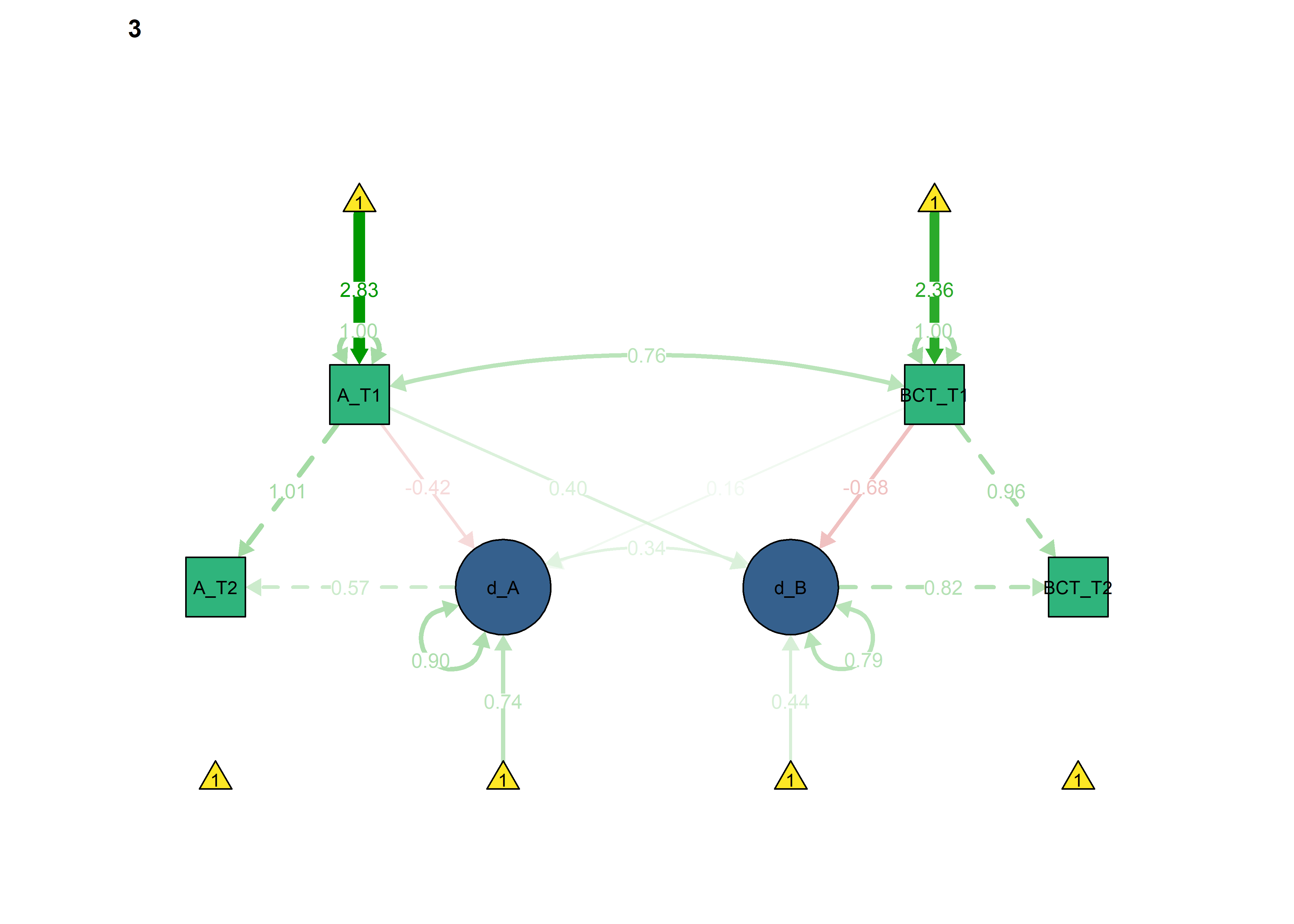
Next, we constrain the parameters which ought to differ across intervention and control groups, to see if model fit changes.
Mean Autonomous change forced as equal
First, constrain the intercept of the change score in Autonomous.
data_BLCS <- df %>% dplyr::select(
  intervention,
  Autonomous_T1 = PA_autonomous_T1,
  Autonomous_T2 = PA_autonomous_T3,
  frqbct_T1 = PA_frqbct_T1,
  frqbct_T2 = PA_frqbct_T3,
  agrbct_T1 = PA_agrbct_T1,
  agrbct_T2 = PA_agrbct_T3) %>%
  rowwise() %>%
  dplyr::mutate(BCTs_T1 = mean(c(frqbct_T1, agrbct_T1), na.rm = TRUE),
                BCTs_T2 = mean(c(frqbct_T2, agrbct_T2), na.rm = TRUE)) %>%
  dplyr::select(-contains("frq"), -contains("agr"))


#Fit the Bivariate Latent Change Score model to simulated data
BLCS_constrained_equalChanges_autonomous <- '

Autonomous_T2 ~ 1 * Autonomous_T1       # This parameter regresses Autonomous_T2 perfectly on Autonomous_T1
d_Autonomous1 =~ 1 * Autonomous_T2      # This defines the latent change score factor as measured perfectly by scores on Autonomous_T2
d_Autonomous1 ~ c(d_autint, d_autint) * 1                     # This estimates the intercept of the change score
Autonomous_T1 ~  c(autint, autint) * 1  # This constrains the intercept of Autonomous_T1 to be identical across intervention and control groups
Autonomous_T2 ~ 0 * 1                   # This constrains the intercept of Autonomous_T2 to 0

BCTs_T2 ~ 1 * BCTs_T1     # This parameter regresses BCTs_T2 perfectly on BCTs_T1
d_BCTs1 =~ 1 * BCTs_T2    # This defines the latent change score factor as measured perfectly by scores on BCTs_T2
BCTs_T2 ~ 0 * 1           # This line constrains the intercept of BCTs_T2 to 0
BCTs_T2 ~~ 0 * BCTs_T2    # This fixes the variance of the BCTs_T1 to 0

d_Autonomous1 ~~  d_Autonomous1                     # This estimates the variance of the change scores
Autonomous_T1 ~~ c(autvar, autvar) * Autonomous_T1  # This estimates the variance of the Autonomous_T1
Autonomous_T2 ~~ 0 * Autonomous_T2                  # This fixes the variance of the Autonomous_T2 to 0

d_BCTs1 ~ 1                            # This estimates the intercept of the change score
BCTs_T1 ~ c(bctint, bctint) * 1        # This estimates the intercept of BCTs_T1
d_BCTs1 ~~ d_BCTs1                     # This estimates the variance of the change scores
BCTs_T1 ~~ c(bctvar, bctvar) * BCTs_T1 # This estimates the variance of BCTs_T1

d_BCTs1 ~ Autonomous_T1 + BCTs_T1       # This estimates the autonomous to BCT coupling parameter and the BCT (T1) to BCT (T2) self-feedback
d_Autonomous1 ~ BCTs_T1 + Autonomous_T1 # This estimates the BCT to autonomous coupling parameter and the autonomous (T1) to autonomous (T2) self-feedback

Autonomous_T1 ~~ c(autbct_cov, autbct_cov) * BCTs_T1                      # This estimates the Autonomous_T1 BCTs_T1 covariance
d_Autonomous1 ~~ d_BCTs1                      # This estimates the d_Autonomous and d_BCTs covariance
'

fitBLCS_constrained_equalChanges_autonomous <- lavaan::lavaan(BLCS_constrained_equalChanges_autonomous,
                          data = data_BLCS,
                          estimator = 'mlr',
                          fixed.x = FALSE,
                          group = "intervention",
                          missing = 'fiml')
## Warning in lav_data_full(data = data, group = group, cluster = cluster, : lavaan WARNING: group variable 'intervention' contains missing values
## Warning in lav_data_full(data = data, group = group, cluster = cluster, : lavaan WARNING: some cases are empty and will be ignored:
##   86

lavaan::summary(fitBLCS_constrained_equalChanges_autonomous, fit.measures = TRUE, standardized = TRUE, rsquare = TRUE)
## lavaan (0.5-23.1097) converged normally after  65 iterations
##
##   Number of observations per group
##   1                                                581
##   0                                                502
##
##   Number of missing patterns per group
##   1                                                  8
##   0                                                  7
##
##   Estimator                                         ML      Robust
##   Minimum Function Test Statistic                8.466       8.933
##   Degrees of freedom                                 6           6
##   P-value (Chi-square)                           0.206       0.177
##   Scaling correction factor                                  0.948
##     for the Yuan-Bentler correction
##
## Chi-square for each group:
##
##   1                                              4.125       4.352
##   0                                              4.341       4.581
##
## Model test baseline model:
##
##   Minimum Function Test Statistic             1778.504    1178.148
##   Degrees of freedom                                12          12
##   P-value                                        0.000       0.000
##
## User model versus baseline model:
##
##   Comparative Fit Index (CFI)                    0.999       0.997
##   Tucker-Lewis Index (TLI)                       0.997       0.995
##
##   Robust Comparative Fit Index (CFI)                         0.998
##   Robust Tucker-Lewis Index (TLI)                            0.997
##
## Loglikelihood and Information Criteria:
##
##   Loglikelihood user model (H0)              -5058.137   -5058.137
##   Scaling correction factor                                  0.942
##     for the MLR correction
##   Loglikelihood unrestricted model (H1)      -5053.904   -5053.904
##   Scaling correction factor                                  1.145
##     for the MLR correction
##
##   Number of free parameters                         22          22
##   Akaike (AIC)                               10160.273   10160.273
##   Bayesian (BIC)                             10269.998   10269.998
##   Sample-size adjusted Bayesian (BIC)        10200.121   10200.121
##
## Root Mean Square Error of Approximation:
##
##   RMSEA                                          0.028       0.030
##   90 Percent Confidence Interval          0.000  0.067       0.000  0.069
##   P-value RMSEA <= 0.05                          0.795       0.759
##
##   Robust RMSEA                                               0.029
##   90 Percent Confidence Interval                             0.000  0.066
##
## Standardized Root Mean Square Residual:
##
##   SRMR                                           0.032       0.032
##
## Parameter Estimates:
##
##   Information                                 Observed
##   Standard Errors                   Robust.huber.white
##
##
## Group 1 [1]:
##
## Latent Variables:
##                    Estimate  Std.Err  z-value  P(>|z|)   Std.lv  Std.all
##   d_Autonomous1 =~
##     Autonomous_T2     1.000                               0.801    0.741
##   d_BCTs1 =~
##     BCTs_T2           1.000                               1.011    0.799
##
## Regressions:
##                    Estimate  Std.Err  z-value  P(>|z|)   Std.lv  Std.all
##   Autonomous_T2 ~
##     Autonomous_T1     1.000                               1.000    0.974
##   BCTs_T2 ~
##     BCTs_T1           1.000                               1.000    0.909
##   d_BCTs1 ~
##     Autonomous_T1     0.241    0.058    4.179    0.000    0.239    0.251
##     BCTs_T1          -0.416    0.062   -6.744    0.000   -0.412   -0.474
##   d_Autonomous1 ~
##     BCTs_T1           0.140    0.047    2.996    0.003    0.175    0.201
##     Autonomous_T1    -0.357    0.045   -7.954    0.000   -0.445   -0.469
##
## Covariances:
##                    Estimate  Std.Err  z-value  P(>|z|)   Std.lv  Std.all
##   Autonomous_T1 ~~
##     BCTs_T1 (atb_)    0.743    0.037   20.053    0.000    0.743    0.614
##  .d_Autonomous1 ~~
##    .d_BCTs1           0.202    0.041    4.878    0.000    0.291    0.291
##
## Intercepts:
##                    Estimate  Std.Err  z-value  P(>|z|)   Std.lv  Std.all
##    .d_Atnm1 (d_tn)    0.853    0.082   10.429    0.000    1.065    1.065
##     Atnm_T1 (atnt)    3.411    0.032  106.563    0.000    3.411    3.241
##    .Atnm_T2           0.000                               0.000    0.000
##    .BCTs_T2           0.000                               0.000    0.000
##    .d_BCTs1           0.572    0.126    4.535    0.000    0.566    0.566
##     BCTs_T1 (bctn)    2.818    0.035   80.404    0.000    2.818    2.450
##
## Variances:
##                    Estimate  Std.Err  z-value  P(>|z|)   Std.lv  Std.all
##    .BCTs_T2           0.000                               0.000    0.000
##    .d_Atnm1           0.549    0.052   10.640    0.000    0.856    0.856
##     Atnm_T1 (atvr)    1.108    0.039   28.244    0.000    1.108    1.000
##    .Atnm_T2           0.000                               0.000    0.000
##    .d_BCTs1           0.877    0.062   14.147    0.000    0.858    0.858
##     BCTs_T1 (bctv)    1.324    0.050   26.594    0.000    1.324    1.000
##
## R-Square:
##                    Estimate
##     BCTs_T2           1.000
##     d_Autonomous1     0.144
##     Autonomous_T2     1.000
##     d_BCTs1           0.142
##
##
## Group 2 [0]:
##
## Latent Variables:
##                    Estimate  Std.Err  z-value  P(>|z|)   Std.lv  Std.all
##   d_Autonomous1 =~
##     Autonomous_T2     1.000                               0.686    0.677
##   d_BCTs1 =~
##     BCTs_T2           1.000                               1.034    0.882
##
## Regressions:
##                    Estimate  Std.Err  z-value  P(>|z|)   Std.lv  Std.all
##   Autonomous_T2 ~
##     Autonomous_T1     1.000                               1.000    1.040
##   BCTs_T2 ~
##     BCTs_T1           1.000                               1.000    0.982
##   d_BCTs1 ~
##     Autonomous_T1     0.248    0.061    4.070    0.000    0.240    0.252
##     BCTs_T1          -0.524    0.059   -8.883    0.000   -0.507   -0.583
##   d_Autonomous1 ~
##     BCTs_T1           0.106    0.042    2.499    0.012    0.154    0.178
##     Autonomous_T1    -0.321    0.042   -7.612    0.000   -0.468   -0.493
##
## Covariances:
##                    Estimate  Std.Err  z-value  P(>|z|)   Std.lv  Std.all
##   Autonomous_T1 ~~
##     BCTs_T1 (atb_)    0.743    0.037   20.053    0.000    0.743    0.614
##  .d_Autonomous1 ~~
##    .d_BCTs1           0.100    0.032    3.120    0.002    0.176    0.176
##
## Intercepts:
##                    Estimate  Std.Err  z-value  P(>|z|)   Std.lv  Std.all
##    .d_Atnm1 (d_tn)    0.853    0.082   10.429    0.000    1.244    1.244
##     Atnm_T1 (atnt)    3.411    0.032  106.563    0.000    3.411    3.241
##    .Atnm_T2           0.000                               0.000    0.000
##    .BCTs_T2           0.000                               0.000    0.000
##    .d_BCTs1           0.668    0.142    4.700    0.000    0.646    0.646
##     BCTs_T1 (bctn)    2.818    0.035   80.404    0.000    2.818    2.450
##
## Variances:
##                    Estimate  Std.Err  z-value  P(>|z|)   Std.lv  Std.all
##    .BCTs_T2           0.000                               0.000    0.000
##    .d_Atnm1           0.392    0.032   12.329    0.000    0.833    0.833
##     Atnm_T1 (atvr)    1.108    0.039   28.244    0.000    1.108    1.000
##    .Atnm_T2           0.000                               0.000    0.000
##    .d_BCTs1           0.830    0.064   13.045    0.000    0.777    0.777
##     BCTs_T1 (bctv)    1.324    0.050   26.594    0.000    1.324    1.000
##
## R-Square:
##                    Estimate
##     BCTs_T2           1.000
##     d_Autonomous1     0.167
##     Autonomous_T2     1.000
##     d_BCTs1           0.223

lavaan::anova(fitBLCS, fitBLCS_constrained, fitBLCS_constrained_equalChanges_autonomous)
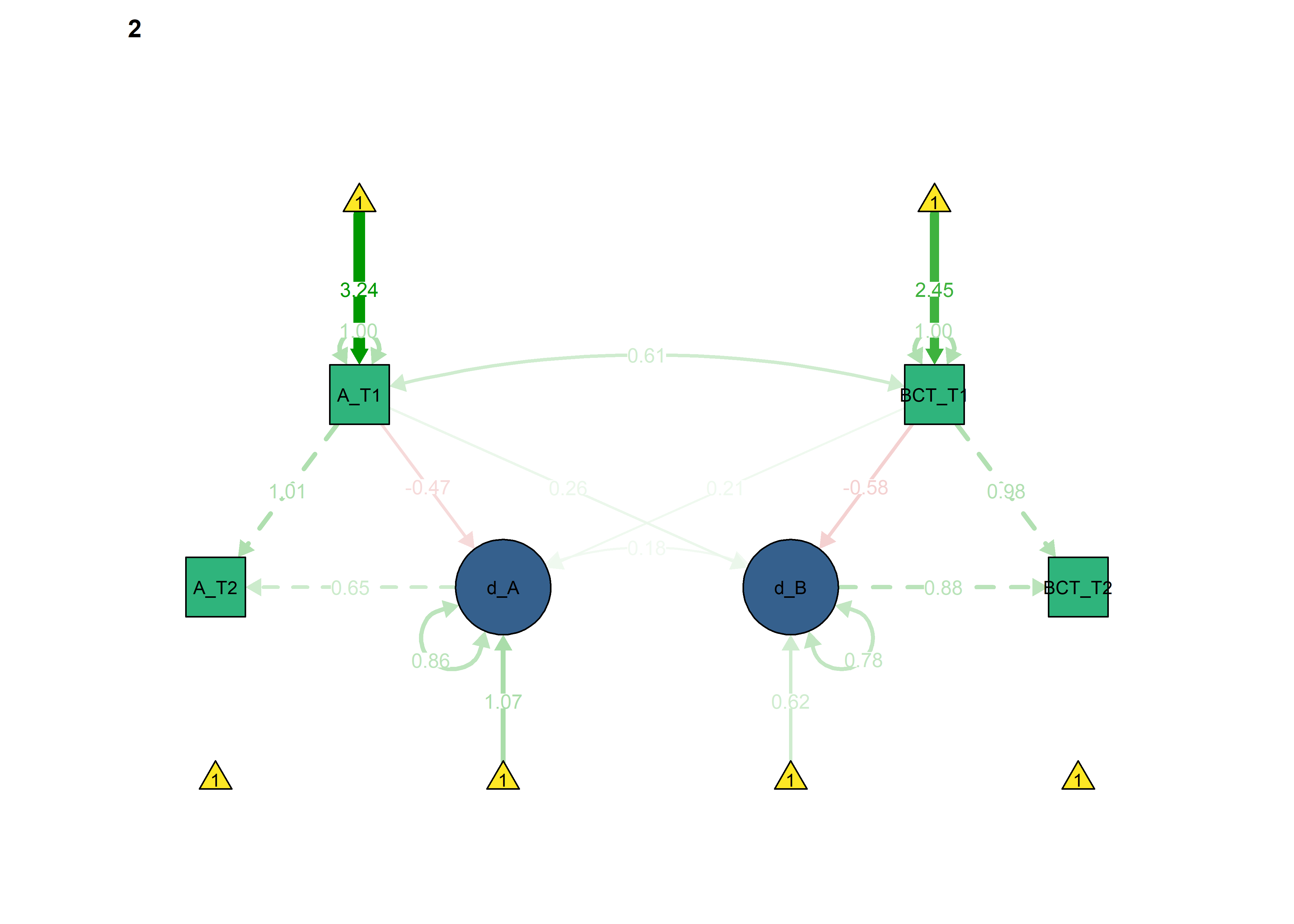
semPlot::semPaths(fitBLCS_constrained_equalChanges_autonomous,
                  what = "std",
                  ask = FALSE,
                  label.cex = .6,
                  label.scale = FALSE,
                  edge.label.cex = 0.75,
                  layout = "tree2",
                  intercepts = TRUE,
                  color = list(lat = viridis::viridis(3, begin = 0.3)[1],
                               man = viridis::viridis(3, begin = 0.3)[2],
                               int = viridis::viridis(3, begin = 0.3)[3]))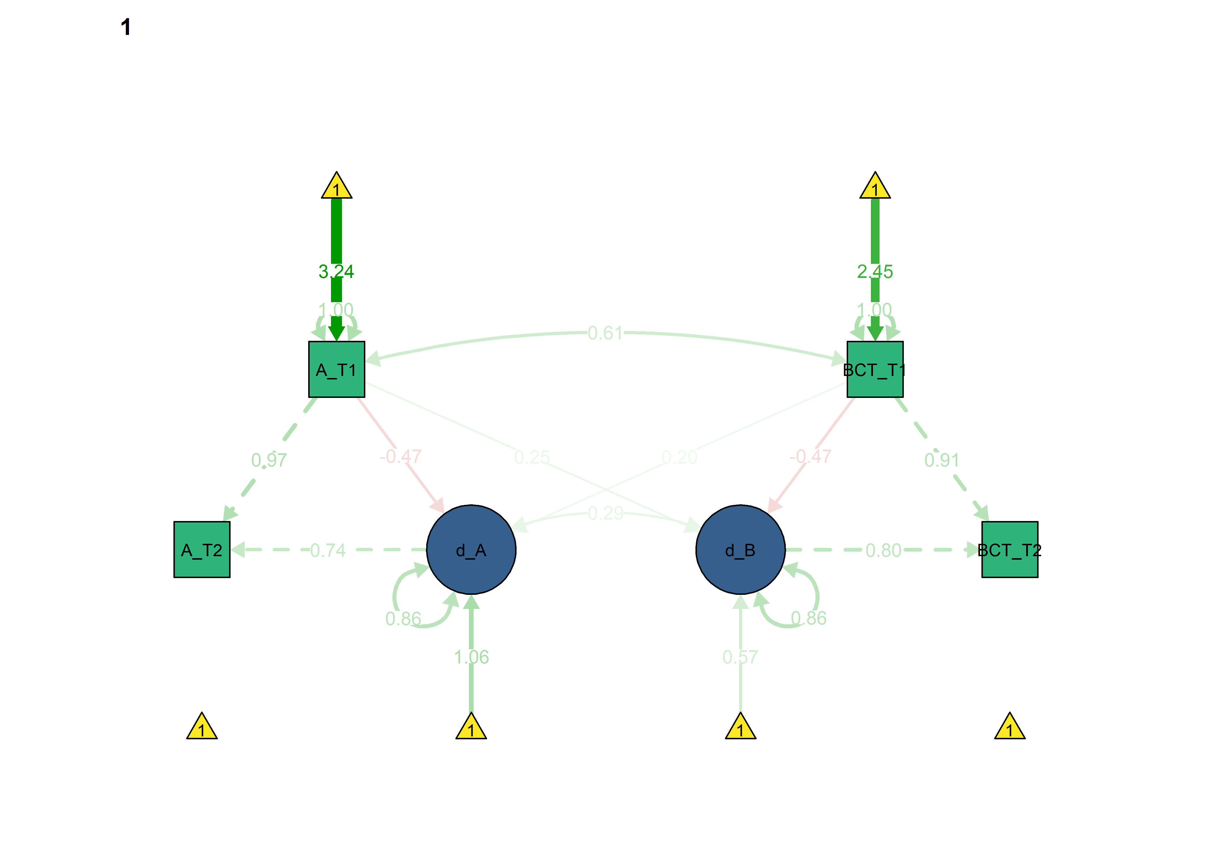
We can see that model fit and out-of-sample prediction gets worse.
Mean BCT change forced as equal
Here we constrain the change in BCTs to be equal across groups:
data_BLCS <- df %>% dplyr::select(
  intervention,
  Autonomous_T1 = PA_autonomous_T1,
  Autonomous_T2 = PA_autonomous_T3,
  frqbct_T1 = PA_frqbct_T1,
  frqbct_T2 = PA_frqbct_T3,
  agrbct_T1 = PA_agrbct_T1,
  agrbct_T2 = PA_agrbct_T3) %>%
  rowwise() %>%
  dplyr::mutate(BCTs_T1 = mean(c(frqbct_T1, agrbct_T1), na.rm = TRUE),
                BCTs_T2 = mean(c(frqbct_T2, agrbct_T2), na.rm = TRUE)) %>%
  dplyr::select(-contains("frq"), -contains("agr"))


#Fit the Bivariate Latent Change Score model to simulated data
BLCS_constrained_equalChanges_bcts <- '

Autonomous_T2 ~ 1 * Autonomous_T1     # This parameter regresses Autonomous_T2 perfectly on Autonomous_T1
d_Autonomous1 =~ 1 * Autonomous_T2    # This defines the latent change score factor as measured perfectly by scores on Autonomous_T2
d_Autonomous1 ~ 1                     # This estimates the intercept of the change score
Autonomous_T1 ~  c(autint, autint)*1  # This constrains the intercept of Autonomous_T1 to be identical across intervention and control groups
Autonomous_T2 ~ 0 * 1                 # This constrains the intercept of Autonomous_T2 to 0

BCTs_T2 ~ 1 * BCTs_T1     # This parameter regresses BCTs_T2 perfectly on BCTs_T1
d_BCTs1 =~ 1 * BCTs_T2    # This defines the latent change score factor as measured perfectly by scores on BCTs_T2
BCTs_T2 ~ 0 * 1           # This line constrains the intercept of BCTs_T2 to 0
BCTs_T2 ~~ 0 * BCTs_T2    # This fixes the variance of the BCTs_T1 to 0

d_Autonomous1 ~~  d_Autonomous1                     # This estimates the variance of the change scores
Autonomous_T1 ~~ c(autvar, autvar) * Autonomous_T1  # This estimates the variance of the Autonomous_T1
Autonomous_T2 ~~ 0 * Autonomous_T2                  # This fixes the variance of the Autonomous_T2 to 0

d_BCTs1 ~ c(d_bctint, d_bctint) * 1                            # This estimates the intercept of the change score
BCTs_T1 ~ c(bctint, bctint) * 1        # This estimates the intercept of BCTs_T1
d_BCTs1 ~~ d_BCTs1                     # This estimates the variance of the change scores
BCTs_T1 ~~ c(bctvar, bctvar) * BCTs_T1 # This estimates the variance of BCTs_T1

d_BCTs1 ~ Autonomous_T1 + BCTs_T1       # This estimates the autonomous to BCT coupling parameter and the BCT (T1) to BCT (T2) self-feedback
d_Autonomous1 ~ BCTs_T1 + Autonomous_T1 # This estimates the BCT to autonomous coupling parameter and the autonomous (T1) to autonomous (T2) self-feedback

Autonomous_T1 ~~ c(autbct_cov, autbct_cov) * BCTs_T1                      # This estimates the Autonomous_T1 BCTs_T1 covariance
d_Autonomous1 ~~ d_BCTs1                      # This estimates the d_Autonomous and d_BCTs covariance
'

fitBLCS_constrained_equalChanges_bcts <- lavaan::lavaan(BLCS_constrained_equalChanges_bcts,
                          data = data_BLCS,
                          estimator = 'mlr',
                          fixed.x = FALSE,
                          group = "intervention",
                          missing = 'fiml')
## Warning in lav_data_full(data = data, group = group, cluster = cluster, : lavaan WARNING: group variable 'intervention' contains missing values
## Warning in lav_data_full(data = data, group = group, cluster = cluster, : lavaan WARNING: some cases are empty and will be ignored:
##   86

lavaan::summary(fitBLCS_constrained_equalChanges_bcts, fit.measures = TRUE, standardized = TRUE, rsquare = TRUE)
## lavaan (0.5-23.1097) converged normally after  52 iterations
##
##   Number of observations per group
##   1                                                581
##   0                                                502
##
##   Number of missing patterns per group
##   1                                                  8
##   0                                                  7
##
##   Estimator                                         ML      Robust
##   Minimum Function Test Statistic                5.542       6.082
##   Degrees of freedom                                 6           6
##   P-value (Chi-square)                           0.476       0.414
##   Scaling correction factor                                  0.911
##     for the Yuan-Bentler correction
##
## Chi-square for each group:
##
##   1                                              2.525       2.771
##   0                                              3.017       3.311
##
## Model test baseline model:
##
##   Minimum Function Test Statistic             1778.504    1178.148
##   Degrees of freedom                                12          12
##   P-value                                        0.000       0.000
##
## User model versus baseline model:
##
##   Comparative Fit Index (CFI)                    1.000       1.000
##   Tucker-Lewis Index (TLI)                       1.001       1.000
##
##   Robust Comparative Fit Index (CFI)                         1.000
##   Robust Tucker-Lewis Index (TLI)                            1.000
##
## Loglikelihood and Information Criteria:
##
##   Loglikelihood user model (H0)              -5056.675   -5056.675
##   Scaling correction factor                                  0.950
##     for the MLR correction
##   Loglikelihood unrestricted model (H1)      -5053.904   -5053.904
##   Scaling correction factor                                  1.145
##     for the MLR correction
##
##   Number of free parameters                         22          22
##   Akaike (AIC)                               10157.350   10157.350
##   Bayesian (BIC)                             10267.074   10267.074
##   Sample-size adjusted Bayesian (BIC)        10197.198   10197.198
##
## Root Mean Square Error of Approximation:
##
##   RMSEA                                          0.000       0.005
##   90 Percent Confidence Interval          0.000  0.053       0.000  0.058
##   P-value RMSEA <= 0.05                          0.931       0.898
##
##   Robust RMSEA                                               0.005
##   90 Percent Confidence Interval                             0.000  0.054
##
## Standardized Root Mean Square Residual:
##
##   SRMR                                           0.027       0.027
##
## Parameter Estimates:
##
##   Information                                 Observed
##   Standard Errors                   Robust.huber.white
##
##
## Group 1 [1]:
##
## Latent Variables:
##                    Estimate  Std.Err  z-value  P(>|z|)   Std.lv  Std.all
##   d_Autonomous1 =~
##     Autonomous_T2     1.000                               0.814    0.776
##   d_BCTs1 =~
##     BCTs_T2           1.000                               1.012    0.806
##
## Regressions:
##                    Estimate  Std.Err  z-value  P(>|z|)   Std.lv  Std.all
##   Autonomous_T2 ~
##     Autonomous_T1     1.000                               1.000    1.003
##   BCTs_T2 ~
##     BCTs_T1           1.000                               1.000    0.916
##   d_BCTs1 ~
##     Autonomous_T1     0.228    0.055    4.178    0.000    0.226    0.237
##     BCTs_T1          -0.420    0.061   -6.827    0.000   -0.415   -0.477
##   d_Autonomous1 ~
##     BCTs_T1           0.131    0.046    2.849    0.004    0.161    0.186
##     Autonomous_T1    -0.390    0.051   -7.594    0.000   -0.480   -0.505
##
## Covariances:
##                    Estimate  Std.Err  z-value  P(>|z|)   Std.lv  Std.all
##   Autonomous_T1 ~~
##     BCTs_T1 (atb_)    0.743    0.037   20.056    0.000    0.743    0.614
##  .d_Autonomous1 ~~
##    .d_BCTs1           0.202    0.041    4.896    0.000    0.291    0.291
##
## Intercepts:
##                    Estimate  Std.Err  z-value  P(>|z|)   Std.lv  Std.all
##    .d_Atnm1           1.004    0.125    8.025    0.000    1.233    1.233
##     Atnm_T1 (atnt)    3.411    0.032  106.562    0.000    3.411    3.241
##    .Atnm_T2           0.000                               0.000    0.000
##    .BCTs_T2           0.000                               0.000    0.000
##    .d_BCTs1 (d_bc)    0.631    0.097    6.508    0.000    0.623    0.623
##     BCTs_T1 (bctn)    2.818    0.035   80.404    0.000    2.818    2.450
##
## Variances:
##                    Estimate  Std.Err  z-value  P(>|z|)   Std.lv  Std.all
##    .BCTs_T2           0.000                               0.000    0.000
##    .d_Atnm1           0.547    0.051   10.768    0.000    0.826    0.826
##     Atnm_T1 (atvr)    1.108    0.039   28.244    0.000    1.108    1.000
##    .Atnm_T2           0.000                               0.000    0.000
##    .d_BCTs1           0.877    0.062   14.166    0.000    0.855    0.855
##     BCTs_T1 (bctv)    1.324    0.050   26.596    0.000    1.324    1.000
##
## R-Square:
##                    Estimate
##     BCTs_T2           1.000
##     d_Autonomous1     0.174
##     Autonomous_T2     1.000
##     d_BCTs1           0.145
##
##
## Group 2 [0]:
##
## Latent Variables:
##                    Estimate  Std.Err  z-value  P(>|z|)   Std.lv  Std.all
##   d_Autonomous1 =~
##     Autonomous_T2     1.000                               0.673    0.648
##   d_BCTs1 =~
##     BCTs_T2           1.000                               1.032    0.877
##
## Regressions:
##                    Estimate  Std.Err  z-value  P(>|z|)   Std.lv  Std.all
##   Autonomous_T2 ~
##     Autonomous_T1     1.000                               1.000    1.013
##   BCTs_T2 ~
##     BCTs_T1           1.000                               1.000    0.977
##   d_BCTs1 ~
##     Autonomous_T1     0.256    0.055    4.681    0.000    0.248    0.261
##     BCTs_T1          -0.523    0.059   -8.849    0.000   -0.506   -0.583
##   d_Autonomous1 ~
##     BCTs_T1           0.112    0.043    2.623    0.009    0.166    0.191
##     Autonomous_T1    -0.293    0.044   -6.614    0.000   -0.435   -0.457
##
## Covariances:
##                    Estimate  Std.Err  z-value  P(>|z|)   Std.lv  Std.all
##   Autonomous_T1 ~~
##     BCTs_T1 (atb_)    0.743    0.037   20.056    0.000    0.743    0.614
##  .d_Autonomous1 ~~
##    .d_BCTs1           0.100    0.032    3.121    0.002    0.175    0.175
##
## Intercepts:
##                    Estimate  Std.Err  z-value  P(>|z|)   Std.lv  Std.all
##    .d_Atnm1           0.728    0.102    7.140    0.000    1.082    1.082
##     Atnm_T1 (atnt)    3.411    0.032  106.562    0.000    3.411    3.241
##    .Atnm_T2           0.000                               0.000    0.000
##    .BCTs_T2           0.000                               0.000    0.000
##    .d_BCTs1 (d_bc)    0.631    0.097    6.508    0.000    0.611    0.611
##     BCTs_T1 (bctn)    2.818    0.035   80.404    0.000    2.818    2.450
##
## Variances:
##                    Estimate  Std.Err  z-value  P(>|z|)   Std.lv  Std.all
##    .BCTs_T2           0.000                               0.000    0.000
##    .d_Atnm1           0.390    0.032   12.252    0.000    0.861    0.861
##     Atnm_T1 (atvr)    1.108    0.039   28.244    0.000    1.108    1.000
##    .Atnm_T2           0.000                               0.000    0.000
##    .d_BCTs1           0.830    0.064   13.045    0.000    0.779    0.779
##     BCTs_T1 (bctv)    1.324    0.050   26.596    0.000    1.324    1.000
##
## R-Square:
##                    Estimate
##     BCTs_T2           1.000
##     d_Autonomous1     0.139
##     Autonomous_T2     1.000
##     d_BCTs1           0.221

lavaan::anova(fitBLCS, fitBLCS_constrained, fitBLCS_constrained_equalChanges_bcts)
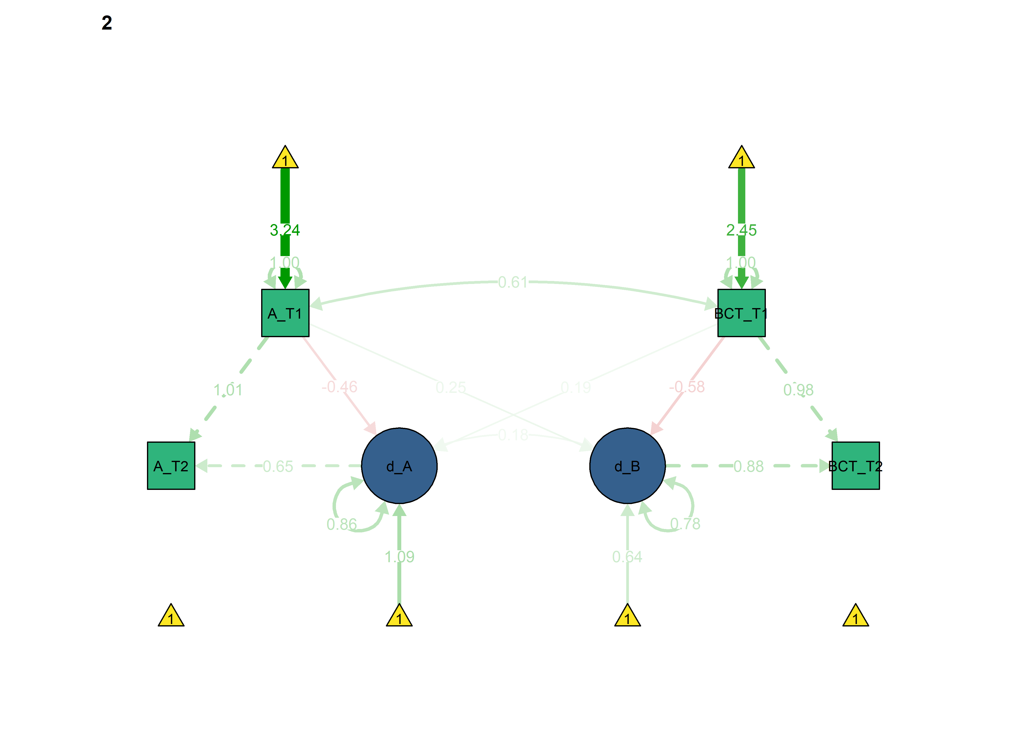
semPlot::semPaths(fitBLCS_constrained_equalChanges_bcts,
                  what = "std",
                  ask = FALSE,
                  label.cex = .6,
                  label.scale = FALSE,
                  edge.label.cex = 0.75,
                  layout = "tree2",
                  intercepts = TRUE,
                  color = list(lat = viridis::viridis(3, begin = 0.3)[1],
                               man = viridis::viridis(3, begin = 0.3)[2],
                               int = viridis::viridis(3, begin = 0.3)[3]))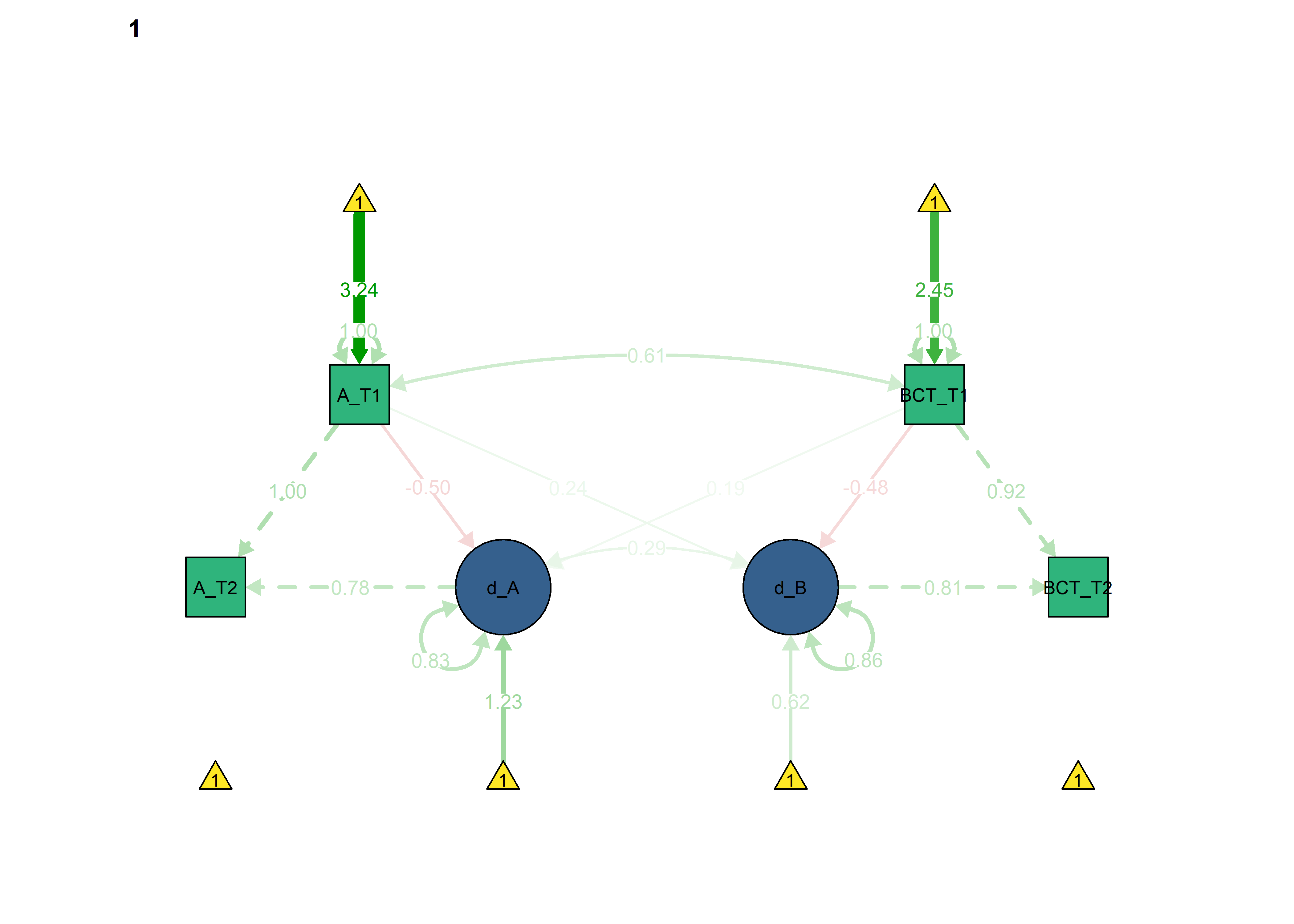

BCT -> Autonomous forced as equal
What if the intervention changed the coupling effect?
Here we constrain the coupling from BCTs to autonomous motivation:
data_BLCS <- df %>% dplyr::select(
  intervention,
  Autonomous_T1 = PA_autonomous_T1,
  Autonomous_T2 = PA_autonomous_T3,
  frqbct_T1 = PA_frqbct_T1,
  frqbct_T2 = PA_frqbct_T3,
  agrbct_T1 = PA_agrbct_T1,
  agrbct_T2 = PA_agrbct_T3) %>%
  rowwise() %>%
  dplyr::mutate(BCTs_T1 = mean(c(frqbct_T1, agrbct_T1), na.rm = TRUE),
                BCTs_T2 = mean(c(frqbct_T2, agrbct_T2), na.rm = TRUE)) %>%
  dplyr::select(-contains("frq"), -contains("agr"))


#Fit the Bivariate Latent Change Score model to simulated data
BLCS_constrained_eqCoupling_bctToAut <- '

Autonomous_T2 ~ 1 * Autonomous_T1     # This parameter regresses Autonomous_T2 perfectly on Autonomous_T1
d_Autonomous1 =~ 1 * Autonomous_T2    # This defines the latent change score factor as measured perfectly by scores on Autonomous_T2
d_Autonomous1 ~ 1                     # This estimates the intercept of the change score
Autonomous_T1 ~  c(autint, autint)*1  # This constrains the intercept of Autonomous_T1 to be identical across intervention and control groups
Autonomous_T2 ~ 0 * 1                 # This constrains the intercept of Autonomous_T2 to 0

BCTs_T2 ~ 1 * BCTs_T1     # This parameter regresses BCTs_T2 perfectly on BCTs_T1
d_BCTs1 =~ 1 * BCTs_T2    # This defines the latent change score factor as measured perfectly by scores on BCTs_T2
BCTs_T2 ~ 0 * 1           # This line constrains the intercept of BCTs_T2 to 0
BCTs_T2 ~~ 0 * BCTs_T2    # This fixes the variance of the BCTs_T1 to 0

d_Autonomous1 ~~  d_Autonomous1                     # This estimates the variance of the change scores
Autonomous_T1 ~~ c(autvar, autvar) * Autonomous_T1  # This estimates the variance of the Autonomous_T1
Autonomous_T2 ~~ 0 * Autonomous_T2                  # This fixes the variance of the Autonomous_T2 to 0

d_BCTs1 ~ 1                            # This estimates the intercept of the change score
BCTs_T1 ~ c(bctint, bctint) * 1        # This estimates the intercept of BCTs_T1
d_BCTs1 ~~ d_BCTs1                     # This estimates the variance of the change scores
BCTs_T1 ~~ c(bctvar, bctvar) * BCTs_T1 # This estimates the variance of BCTs_T1

d_BCTs1 ~ Autonomous_T1 + BCTs_T1       # This estimates the autonomous to BCT coupling parameter and the BCT (T1) to BCT (T2) self-feedback
d_Autonomous1 ~ c(d_bctaut, d_bctaut) * BCTs_T1 + Autonomous_T1 # This estimates the BCT to autonomous coupling parameter and the autonomous (T1) to autonomous (T2) self-feedback

Autonomous_T1 ~~ c(autbct_cov, autbct_cov) * BCTs_T1                      # This estimates the Autonomous_T1 BCTs_T1 covariance
d_Autonomous1 ~~ d_BCTs1                      # This estimates the d_Autonomous and d_BCTs covariance
'

fitBLCS_constrained_eqCoupling_bctToAut <- lavaan::lavaan(BLCS_constrained_eqCoupling_bctToAut,
                          data = data_BLCS,
                          estimator = 'mlr',
                          fixed.x = FALSE,
                          group = "intervention",
                          missing = 'fiml')
## Warning in lav_data_full(data = data, group = group, cluster = cluster, : lavaan WARNING: group variable 'intervention' contains missing values
## Warning in lav_data_full(data = data, group = group, cluster = cluster, : lavaan WARNING: some cases are empty and will be ignored:
##   86

lavaan::summary(fitBLCS_constrained_eqCoupling_bctToAut, fit.measures = TRUE, standardized = TRUE, rsquare = TRUE)
## lavaan (0.5-23.1097) converged normally after  56 iterations
##
##   Number of observations per group
##   1                                                581
##   0                                                502
##
##   Number of missing patterns per group
##   1                                                  8
##   0                                                  7
##
##   Estimator                                         ML      Robust
##   Minimum Function Test Statistic                5.686       5.567
##   Degrees of freedom                                 6           6
##   P-value (Chi-square)                           0.459       0.473
##   Scaling correction factor                                  1.021
##     for the Yuan-Bentler correction
##
## Chi-square for each group:
##
##   1                                              2.603       2.549
##   0                                              3.083       3.018
##
## Model test baseline model:
##
##   Minimum Function Test Statistic             1778.504    1178.148
##   Degrees of freedom                                12          12
##   P-value                                        0.000       0.000
##
## User model versus baseline model:
##
##   Comparative Fit Index (CFI)                    1.000       1.000
##   Tucker-Lewis Index (TLI)                       1.000       1.001
##
##   Robust Comparative Fit Index (CFI)                         1.000
##   Robust Tucker-Lewis Index (TLI)                            1.001
##
## Loglikelihood and Information Criteria:
##
##   Loglikelihood user model (H0)              -5056.747   -5056.747
##   Scaling correction factor                                  0.926
##     for the MLR correction
##   Loglikelihood unrestricted model (H1)      -5053.904   -5053.904
##   Scaling correction factor                                  1.145
##     for the MLR correction
##
##   Number of free parameters                         22          22
##   Akaike (AIC)                               10157.494   10157.494
##   Bayesian (BIC)                             10267.218   10267.218
##   Sample-size adjusted Bayesian (BIC)        10197.342   10197.342
##
## Root Mean Square Error of Approximation:
##
##   RMSEA                                          0.000       0.000
##   90 Percent Confidence Interval          0.000  0.054       0.000  0.053
##   P-value RMSEA <= 0.05                          0.926       0.932
##
##   Robust RMSEA                                               0.000
##   90 Percent Confidence Interval                             0.000  0.054
##
## Standardized Root Mean Square Residual:
##
##   SRMR                                           0.026       0.026
##
## Parameter Estimates:
##
##   Information                                 Observed
##   Standard Errors                   Robust.huber.white
##
##
## Group 1 [1]:
##
## Latent Variables:
##                    Estimate  Std.Err  z-value  P(>|z|)   Std.lv  Std.all
##   d_Autonomous1 =~
##     Autonomous_T2     1.000                               0.813    0.775
##   d_BCTs1 =~
##     BCTs_T2           1.000                               1.014    0.808
##
## Regressions:
##                    Estimate  Std.Err  z-value  P(>|z|)   Std.lv  Std.all
##   Autonomous_T2 ~
##     Atnm_T1           1.000                               1.000    1.004
##   BCTs_T2 ~
##     BCTs_T1           1.000                               1.000    0.917
##   d_BCTs1 ~
##     Atnm_T1           0.232    0.057    4.044    0.000    0.229    0.241
##     BCTs_T1          -0.423    0.060   -7.066    0.000   -0.418   -0.481
##   d_Autonomous1 ~
##     BCTs_T1 (d_bc)    0.121    0.031    3.868    0.000    0.149    0.171
##     Atnm_T1          -0.383    0.044   -8.686    0.000   -0.472   -0.496
##
## Covariances:
##                    Estimate  Std.Err  z-value  P(>|z|)   Std.lv  Std.all
##   Autonomous_T1 ~~
##     BCTs_T1 (atb_)    0.743    0.037   20.053    0.000    0.743    0.614
##  .d_Autonomous1 ~~
##    .d_BCTs1           0.202    0.041    4.906    0.000    0.291    0.291
##
## Intercepts:
##                    Estimate  Std.Err  z-value  P(>|z|)   Std.lv  Std.all
##    .d_Atnm1           1.009    0.130    7.733    0.000    1.241    1.241
##     Atnm_T1 (atnt)    3.411    0.032  106.563    0.000    3.411    3.241
##    .Atnm_T2           0.000                               0.000    0.000
##    .BCTs_T2           0.000                               0.000    0.000
##    .d_BCTs1           0.629    0.133    4.738    0.000    0.620    0.620
##     BCTs_T1 (bctn)    2.818    0.035   80.404    0.000    2.818    2.450
##
## Variances:
##                    Estimate  Std.Err  z-value  P(>|z|)   Std.lv  Std.all
##    .BCTs_T2           0.000                               0.000    0.000
##    .d_Atnm1           0.547    0.051   10.756    0.000    0.829    0.829
##     Atnm_T1 (atvr)    1.108    0.039   28.244    0.000    1.108    1.000
##    .Atnm_T2           0.000                               0.000    0.000
##    .d_BCTs1           0.877    0.062   14.163    0.000    0.853    0.853
##     BCTs_T1 (bctv)    1.324    0.050   26.595    0.000    1.324    1.000
##
## R-Square:
##                    Estimate
##     BCTs_T2           1.000
##     d_Autonomous1     0.171
##     Autonomous_T2     1.000
##     d_BCTs1           0.147
##
##
## Group 2 [0]:
##
## Latent Variables:
##                    Estimate  Std.Err  z-value  P(>|z|)   Std.lv  Std.all
##   d_Autonomous1 =~
##     Autonomous_T2     1.000                               0.675    0.649
##   d_BCTs1 =~
##     BCTs_T2           1.000                               1.032    0.876
##
## Regressions:
##                    Estimate  Std.Err  z-value  P(>|z|)   Std.lv  Std.all
##   Autonomous_T2 ~
##     Atnm_T1           1.000                               1.000    1.013
##   BCTs_T2 ~
##     BCTs_T1           1.000                               1.000    0.977
##   d_BCTs1 ~
##     Atnm_T1           0.254    0.061    4.184    0.000    0.246    0.259
##     BCTs_T1          -0.521    0.058   -8.904    0.000   -0.505   -0.581
##   d_Autonomous1 ~
##     BCTs_T1 (d_bc)    0.121    0.031    3.868    0.000    0.179    0.206
##     Atnm_T1          -0.299    0.038   -7.848    0.000   -0.443   -0.467
##
## Covariances:
##                    Estimate  Std.Err  z-value  P(>|z|)   Std.lv  Std.all
##   Autonomous_T1 ~~
##     BCTs_T1 (atb_)    0.743    0.037   20.053    0.000    0.743    0.614
##  .d_Autonomous1 ~~
##    .d_BCTs1           0.100    0.032    3.122    0.002    0.176    0.176
##
## Intercepts:
##                    Estimate  Std.Err  z-value  P(>|z|)   Std.lv  Std.all
##    .d_Atnm1           0.725    0.103    7.023    0.000    1.074    1.074
##     Atnm_T1 (atnt)    3.411    0.032  106.563    0.000    3.411    3.241
##    .Atnm_T2           0.000                               0.000    0.000
##    .BCTs_T2           0.000                               0.000    0.000
##    .d_BCTs1           0.635    0.142    4.464    0.000    0.616    0.616
##     BCTs_T1 (bctn)    2.818    0.035   80.404    0.000    2.818    2.450
##
## Variances:
##                    Estimate  Std.Err  z-value  P(>|z|)   Std.lv  Std.all
##    .BCTs_T2           0.000                               0.000    0.000
##    .d_Atnm1           0.390    0.032   12.274    0.000    0.858    0.858
##     Atnm_T1 (atvr)    1.108    0.039   28.244    0.000    1.108    1.000
##    .Atnm_T2           0.000                               0.000    0.000
##    .d_BCTs1           0.830    0.064   13.045    0.000    0.780    0.780
##     BCTs_T1 (bctv)    1.324    0.050   26.595    0.000    1.324    1.000
##
## R-Square:
##                    Estimate
##     BCTs_T2           1.000
##     d_Autonomous1     0.142
##     Autonomous_T2     1.000
##     d_BCTs1           0.220

lavaan::anova(fitBLCS, fitBLCS_constrained, fitBLCS_constrained_eqCoupling_bctToAut)
semPlot::semPaths(fitBLCS_constrained_eqCoupling_bctToAut,
                  what = "std",
                  ask = FALSE,
                  label.cex = .6,
                  label.scale = FALSE,
                  edge.label.cex = 0.75,
                  layout = "tree2",
                  intercepts = TRUE,
                  color = list(lat = viridis::viridis(3, begin = 0.3)[1],
                               man = viridis::viridis(3, begin = 0.3)[2],
                               int = viridis::viridis(3, begin = 0.3)[3]))
Autonomous -> BCT forced as equal
Here we constrain the coupling from autonomous motivation to BCTs:
data_BLCS <- df %>% dplyr::select(
  intervention,
  Autonomous_T1 = PA_autonomous_T1,
  Autonomous_T2 = PA_autonomous_T3,
  frqbct_T1 = PA_frqbct_T1,
  frqbct_T2 = PA_frqbct_T3,
  agrbct_T1 = PA_agrbct_T1,
  agrbct_T2 = PA_agrbct_T3) %>%
  rowwise() %>%
  dplyr::mutate(BCTs_T1 = mean(c(frqbct_T1, agrbct_T1), na.rm = TRUE),
                BCTs_T2 = mean(c(frqbct_T2, agrbct_T2), na.rm = TRUE)) %>%
  dplyr::select(-contains("frq"), -contains("agr"))


#Fit the Bivariate Latent Change Score model to simulated data
BLCS_constrained_eqCoupling_autToBct <- '

Autonomous_T2 ~ 1 * Autonomous_T1     # This parameter regresses Autonomous_T2 perfectly on Autonomous_T1
d_Autonomous1 =~ 1 * Autonomous_T2    # This defines the latent change score factor as measured perfectly by scores on Autonomous_T2
d_Autonomous1 ~ 1                     # This estimates the intercept of the change score
Autonomous_T1 ~  c(autint, autint)*1  # This constrains the intercept of Autonomous_T1 to be identical across intervention and control groups
Autonomous_T2 ~ 0 * 1                 # This constrains the intercept of Autonomous_T2 to 0

BCTs_T2 ~ 1 * BCTs_T1     # This parameter regresses BCTs_T2 perfectly on BCTs_T1
d_BCTs1 =~ 1 * BCTs_T2    # This defines the latent change score factor as measured perfectly by scores on BCTs_T2
BCTs_T2 ~ 0 * 1           # This line constrains the intercept of BCTs_T2 to 0
BCTs_T2 ~~ 0 * BCTs_T2    # This fixes the variance of the BCTs_T1 to 0

d_Autonomous1 ~~  d_Autonomous1                     # This estimates the variance of the change scores
Autonomous_T1 ~~ c(autvar, autvar) * Autonomous_T1  # This estimates the variance of the Autonomous_T1
Autonomous_T2 ~~ 0 * Autonomous_T2                  # This fixes the variance of the Autonomous_T2 to 0

d_BCTs1 ~ 1                            # This estimates the intercept of the change score
BCTs_T1 ~ c(bctint, bctint) * 1        # This estimates the intercept of BCTs_T1
d_BCTs1 ~~ d_BCTs1                     # This estimates the variance of the change scores
BCTs_T1 ~~ c(bctvar, bctvar) * BCTs_T1 # This estimates the variance of BCTs_T1

d_BCTs1 ~ c(d_autbct, d_autbct) * Autonomous_T1 + BCTs_T1       # This estimates the autonomous to BCT coupling parameter and the BCT (T1) to BCT (T2) self-feedback
d_Autonomous1 ~ BCTs_T1 + Autonomous_T1 # This estimates the BCT to autonomous coupling parameter and the autonomous (T1) to autonomous (T2) self-feedback

Autonomous_T1 ~~ c(autbct_cov, autbct_cov) * BCTs_T1                      # This estimates the Autonomous_T1 BCTs_T1 covariance
d_Autonomous1 ~~ d_BCTs1                      # This estimates the d_Autonomous and d_BCTs covariance
'

fitBLCS_constrained_eqCoupling_autToBct <- lavaan::lavaan(BLCS_constrained_eqCoupling_autToBct,
                          data = data_BLCS,
                          estimator = 'mlr',
                          fixed.x = FALSE,
                          group = "intervention",
                          missing = 'fiml')
## Warning in lav_data_full(data = data, group = group, cluster = cluster, : lavaan WARNING: group variable 'intervention' contains missing values
## Warning in lav_data_full(data = data, group = group, cluster = cluster, : lavaan WARNING: some cases are empty and will be ignored:
##   86

lavaan::summary(fitBLCS_constrained_eqCoupling_autToBct, fit.measures = TRUE, standardized = TRUE, rsquare = TRUE)
## lavaan (0.5-23.1097) converged normally after  55 iterations
##
##   Number of observations per group
##   1                                                581
##   0                                                502
##
##   Number of missing patterns per group
##   1                                                  8
##   0                                                  7
##
##   Estimator                                         ML      Robust
##   Minimum Function Test Statistic                5.654       5.769
##   Degrees of freedom                                 6           6
##   P-value (Chi-square)                           0.463       0.450
##   Scaling correction factor                                  0.980
##     for the Yuan-Bentler correction
##
## Chi-square for each group:
##
##   1                                              2.578       2.630
##   0                                              3.076       3.139
##
## Model test baseline model:
##
##   Minimum Function Test Statistic             1778.504    1178.148
##   Degrees of freedom                                12          12
##   P-value                                        0.000       0.000
##
## User model versus baseline model:
##
##   Comparative Fit Index (CFI)                    1.000       1.000
##   Tucker-Lewis Index (TLI)                       1.000       1.000
##
##   Robust Comparative Fit Index (CFI)                         1.000
##   Robust Tucker-Lewis Index (TLI)                            1.000
##
## Loglikelihood and Information Criteria:
##
##   Loglikelihood user model (H0)              -5056.731   -5056.731
##   Scaling correction factor                                  0.935
##     for the MLR correction
##   Loglikelihood unrestricted model (H1)      -5053.904   -5053.904
##   Scaling correction factor                                  1.145
##     for the MLR correction
##
##   Number of free parameters                         22          22
##   Akaike (AIC)                               10157.462   10157.462
##   Bayesian (BIC)                             10267.186   10267.186
##   Sample-size adjusted Bayesian (BIC)        10197.310   10197.310
##
## Root Mean Square Error of Approximation:
##
##   RMSEA                                          0.000       0.000
##   90 Percent Confidence Interval          0.000  0.054       0.000  0.055
##   P-value RMSEA <= 0.05                          0.927       0.920
##
##   Robust RMSEA                                               0.000
##   90 Percent Confidence Interval                             0.000  0.054
##
## Standardized Root Mean Square Residual:
##
##   SRMR                                           0.027       0.027
##
## Parameter Estimates:
##
##   Information                                 Observed
##   Standard Errors                   Robust.huber.white
##
##
## Group 1 [1]:
##
## Latent Variables:
##                    Estimate  Std.Err  z-value  P(>|z|)   Std.lv  Std.all
##   d_Autonomous1 =~
##     Autonomous_T2     1.000                               0.813    0.774
##   d_BCTs1 =~
##     BCTs_T2           1.000                               1.014    0.806
##
## Regressions:
##                    Estimate  Std.Err  z-value  P(>|z|)   Std.lv  Std.all
##   Autonomous_T2 ~
##     Atnm_T1           1.000                               1.000    1.002
##   BCTs_T2 ~
##     BCTs_T1           1.000                               1.000    0.914
##   d_BCTs1 ~
##     Atnm_T1 (d_tb)    0.241    0.042    5.723    0.000    0.238    0.250
##     BCTs_T1          -0.426    0.054   -7.925    0.000   -0.420   -0.483
##   d_Autonomous1 ~
##     BCTs_T1           0.130    0.046    2.851    0.004    0.160    0.184
##     Atnm_T1          -0.387    0.051   -7.609    0.000   -0.477   -0.502
##
## Covariances:
##                    Estimate  Std.Err  z-value  P(>|z|)   Std.lv  Std.all
##   Autonomous_T1 ~~
##     BCTs_T1 (atb_)    0.743    0.037   20.054    0.000    0.743    0.614
##  .d_Autonomous1 ~~
##    .d_BCTs1           0.202    0.041    4.894    0.000    0.291    0.291
##
## Intercepts:
##                    Estimate  Std.Err  z-value  P(>|z|)   Std.lv  Std.all
##    .d_Atnm1           0.998    0.127    7.844    0.000    1.227    1.227
##     Atnm_T1 (atnt)    3.411    0.032  106.562    0.000    3.411    3.241
##    .Atnm_T2           0.000                               0.000    0.000
##    .BCTs_T2           0.000                               0.000    0.000
##    .d_BCTs1           0.604    0.126    4.797    0.000    0.596    0.596
##     BCTs_T1 (bctn)    2.818    0.035   80.407    0.000    2.818    2.450
##
## Variances:
##                    Estimate  Std.Err  z-value  P(>|z|)   Std.lv  Std.all
##    .BCTs_T2           0.000                               0.000    0.000
##    .d_Atnm1           0.547    0.051   10.769    0.000    0.828    0.828
##     Atnm_T1 (atvr)    1.108    0.039   28.243    0.000    1.108    1.000
##    .Atnm_T2           0.000                               0.000    0.000
##    .d_BCTs1           0.877    0.062   14.174    0.000    0.852    0.852
##     BCTs_T1 (bctv)    1.324    0.050   26.595    0.000    1.324    1.000
##
## R-Square:
##                    Estimate
##     BCTs_T2           1.000
##     d_Autonomous1     0.172
##     Autonomous_T2     1.000
##     d_BCTs1           0.148
##
##
## Group 2 [0]:
##
## Latent Variables:
##                    Estimate  Std.Err  z-value  P(>|z|)   Std.lv  Std.all
##   d_Autonomous1 =~
##     Autonomous_T2     1.000                               0.674    0.649
##   d_BCTs1 =~
##     BCTs_T2           1.000                               1.030    0.877
##
## Regressions:
##                    Estimate  Std.Err  z-value  P(>|z|)   Std.lv  Std.all
##   Autonomous_T2 ~
##     Atnm_T1           1.000                               1.000    1.014
##   BCTs_T2 ~
##     BCTs_T1           1.000                               1.000    0.979
##   d_BCTs1 ~
##     Atnm_T1 (d_tb)    0.241    0.042    5.723    0.000    0.234    0.247
##     BCTs_T1          -0.515    0.050  -10.299    0.000   -0.500   -0.575
##   d_Autonomous1 ~
##     BCTs_T1           0.113    0.042    2.664    0.008    0.167    0.192
##     Atnm_T1          -0.294    0.044   -6.712    0.000   -0.437   -0.460
##
## Covariances:
##                    Estimate  Std.Err  z-value  P(>|z|)   Std.lv  Std.all
##   Autonomous_T1 ~~
##     BCTs_T1 (atb_)    0.743    0.037   20.054    0.000    0.743    0.614
##  .d_Autonomous1 ~~
##    .d_BCTs1           0.100    0.032    3.124    0.002    0.176    0.176
##
## Intercepts:
##                    Estimate  Std.Err  z-value  P(>|z|)   Std.lv  Std.all
##    .d_Atnm1           0.732    0.103    7.137    0.000    1.086    1.086
##     Atnm_T1 (atnt)    3.411    0.032  106.562    0.000    3.411    3.241
##    .Atnm_T2           0.000                               0.000    0.000
##    .BCTs_T2           0.000                               0.000    0.000
##    .d_BCTs1           0.661    0.129    5.113    0.000    0.642    0.642
##     BCTs_T1 (bctn)    2.818    0.035   80.407    0.000    2.818    2.450
##
## Variances:
##                    Estimate  Std.Err  z-value  P(>|z|)   Std.lv  Std.all
##    .BCTs_T2           0.000                               0.000    0.000
##    .d_Atnm1           0.390    0.032   12.251    0.000    0.860    0.860
##     Atnm_T1 (atvr)    1.108    0.039   28.243    0.000    1.108    1.000
##    .Atnm_T2           0.000                               0.000    0.000
##    .d_BCTs1           0.831    0.064   13.009    0.000    0.783    0.783
##     BCTs_T1 (bctv)    1.324    0.050   26.595    0.000    1.324    1.000
##
## R-Square:
##                    Estimate
##     BCTs_T2           1.000
##     d_Autonomous1     0.140
##     Autonomous_T2     1.000
##     d_BCTs1           0.217

lavaan::anova(fitBLCS, fitBLCS_constrained, fitBLCS_constrained_eqCoupling_autToBct)
semPlot::semPaths(fitBLCS_constrained_eqCoupling_autToBct,
                  what = "std",
                  ask = FALSE,
                  label.cex = .6,
                  label.scale = FALSE,
                  edge.label.cex = 0.75,
                  layout = "tree2",
                  intercepts = TRUE,
                  color = list(lat = viridis::viridis(3, begin = 0.3)[1],
                               man = viridis::viridis(3, begin = 0.3)[2],
                               int = viridis::viridis(3, begin = 0.3)[3]))
All previous constraints imposed at once
The information criteria seem to imply somewhat better out-of-sample prediction for each of the constraints introduced previously. Here we set all of them:
data_BLCS <- df %>% dplyr::select(
  intervention,
  Autonomous_T1 = PA_autonomous_T1,
  Autonomous_T2 = PA_autonomous_T3,
  frqbct_T1 = PA_frqbct_T1,
  frqbct_T2 = PA_frqbct_T3,
  agrbct_T1 = PA_agrbct_T1,
  agrbct_T2 = PA_agrbct_T3) %>%
  rowwise() %>%
  dplyr::mutate(BCTs_T1 = mean(c(frqbct_T1, agrbct_T1), na.rm = TRUE),
                BCTs_T2 = mean(c(frqbct_T2, agrbct_T2), na.rm = TRUE)) %>%
  dplyr::select(-contains("frq"), -contains("agr"))


#Fit the Bivariate Latent Change Score model to simulated data
BLCS_allConstraints <- '

Autonomous_T2 ~ 1 * Autonomous_T1     # This parameter regresses Autonomous_T2 perfectly on Autonomous_T1
d_Autonomous1 =~ 1 * Autonomous_T2    # This defines the latent change score factor as measured perfectly by scores on Autonomous_T2
d_Autonomous1 ~ c(d_autint, d_autint) * 1                     # This estimates the intercept of the change score
Autonomous_T1 ~  c(autint, autint)*1  # This constrains the intercept of Autonomous_T1 to be identical across intervention and control groups
Autonomous_T2 ~ 0 * 1                 # This constrains the intercept of Autonomous_T2 to 0

BCTs_T2 ~ 1 * BCTs_T1     # This parameter regresses BCTs_T2 perfectly on BCTs_T1
d_BCTs1 =~ 1 * BCTs_T2    # This defines the latent change score factor as measured perfectly by scores on BCTs_T2
BCTs_T2 ~ 0 * 1           # This line constrains the intercept of BCTs_T2 to 0
BCTs_T2 ~~ 0 * BCTs_T2    # This fixes the variance of the BCTs_T1 to 0

d_Autonomous1 ~~  d_Autonomous1                     # This estimates the variance of the change scores
Autonomous_T1 ~~ c(autvar, autvar) * Autonomous_T1  # This estimates the variance of the Autonomous_T1
Autonomous_T2 ~~ 0 * Autonomous_T2                  # This fixes the variance of the Autonomous_T2 to 0

d_BCTs1 ~ c(d_bctint, d_bctint) * 1                            # This estimates the intercept of the change score
BCTs_T1 ~ c(bctint, bctint) * 1        # This estimates the intercept of BCTs_T1
d_BCTs1 ~~ d_BCTs1                     # This estimates the variance of the change scores
BCTs_T1 ~~ c(bctvar, bctvar) * BCTs_T1 # This estimates the variance of BCTs_T1

d_BCTs1 ~ c(d_autbct, d_autbct) * Autonomous_T1 + BCTs_T1       # This estimates the autonomous to BCT coupling parameter and the BCT (T1) to BCT (T2) self-feedback
d_Autonomous1 ~ c(d_bctaut, d_bctaut) * BCTs_T1 + Autonomous_T1 # This estimates the BCT to autonomous coupling parameter and the autonomous (T1) to autonomous (T2) self-feedback

Autonomous_T1 ~~ c(autbct_cov, autbct_cov) * BCTs_T1                      # This estimates the Autonomous_T1 BCTs_T1 covariance
d_Autonomous1 ~~ d_BCTs1                      # This estimates the d_Autonomous and d_BCTs covariance
'

fitBLCS_allConstraints <- lavaan::lavaan(BLCS_allConstraints,
                          data = data_BLCS,
                          estimator = 'mlr',
                          fixed.x = FALSE,
                          group = "intervention",
                          missing = 'fiml')
## Warning in lav_data_full(data = data, group = group, cluster = cluster, : lavaan WARNING: group variable 'intervention' contains missing values
## Warning in lav_data_full(data = data, group = group, cluster = cluster, : lavaan WARNING: some cases are empty and will be ignored:
##   86

lavaan::summary(fitBLCS_allConstraints, fit.measures = TRUE, standardized = TRUE, rsquare = TRUE)
## lavaan (0.5-23.1097) converged normally after  45 iterations
##
##   Number of observations per group
##   1                                                581
##   0                                                502
##
##   Number of missing patterns per group
##   1                                                  8
##   0                                                  7
##
##   Estimator                                         ML      Robust
##   Minimum Function Test Statistic                9.235       8.846
##   Degrees of freedom                                 9           9
##   P-value (Chi-square)                           0.416       0.452
##   Scaling correction factor                                  1.044
##     for the Yuan-Bentler correction
##
## Chi-square for each group:
##
##   1                                              4.473       4.284
##   0                                              4.762       4.562
##
## Model test baseline model:
##
##   Minimum Function Test Statistic             1778.504    1178.148
##   Degrees of freedom                                12          12
##   P-value                                        0.000       0.000
##
## User model versus baseline model:
##
##   Comparative Fit Index (CFI)                    1.000       1.000
##   Tucker-Lewis Index (TLI)                       1.000       1.000
##
##   Robust Comparative Fit Index (CFI)                         1.000
##   Robust Tucker-Lewis Index (TLI)                            1.000
##
## Loglikelihood and Information Criteria:
##
##   Loglikelihood user model (H0)              -5058.521   -5058.521
##   Scaling correction factor                                  0.810
##     for the MLR correction
##   Loglikelihood unrestricted model (H1)      -5053.904   -5053.904
##   Scaling correction factor                                  1.145
##     for the MLR correction
##
##   Number of free parameters                         19          19
##   Akaike (AIC)                               10155.042   10155.042
##   Bayesian (BIC)                             10249.804   10249.804
##   Sample-size adjusted Bayesian (BIC)        10189.457   10189.457
##
## Root Mean Square Error of Approximation:
##
##   RMSEA                                          0.007       0.000
##   90 Percent Confidence Interval          0.000  0.049       0.000  0.047
##   P-value RMSEA <= 0.05                          0.955       0.965
##
##   Robust RMSEA                                               0.000
##   90 Percent Confidence Interval                             0.000  0.049
##
## Standardized Root Mean Square Residual:
##
##   SRMR                                           0.031       0.031
##
## Parameter Estimates:
##
##   Information                                 Observed
##   Standard Errors                   Robust.huber.white
##
##
## Group 1 [1]:
##
## Latent Variables:
##                    Estimate  Std.Err  z-value  P(>|z|)   Std.lv  Std.all
##   d_Autonomous1 =~
##     Autonomous_T2     1.000                               0.798    0.739
##   d_BCTs1 =~
##     BCTs_T2           1.000                               1.018    0.812
##
## Regressions:
##                    Estimate  Std.Err  z-value  P(>|z|)   Std.lv  Std.all
##   Autonomous_T2 ~
##     Atnm_T1           1.000                               1.000    0.974
##   BCTs_T2 ~
##     BCTs_T1           1.000                               1.000    0.918
##   d_BCTs1 ~
##     Atnm_T1 (d_tb)    0.246    0.042    5.811    0.000    0.241    0.254
##     BCTs_T1          -0.436    0.044   -9.813    0.000   -0.428   -0.492
##   d_Autonomous1 ~
##     BCTs_T1 (d_bc)    0.121    0.031    3.876    0.000    0.152    0.175
##     Atnm_T1          -0.342    0.034   -9.992    0.000   -0.429   -0.451
##
## Covariances:
##                    Estimate  Std.Err  z-value  P(>|z|)   Std.lv  Std.all
##   Autonomous_T1 ~~
##     BCTs_T1 (atb_)    0.743    0.037   20.054    0.000    0.743    0.614
##  .d_Autonomous1 ~~
##    .d_BCTs1           0.202    0.041    4.898    0.000    0.291    0.291
##
## Intercepts:
##                    Estimate  Std.Err  z-value  P(>|z|)   Std.lv  Std.all
##    .d_Atnm1 (d_tn)    0.855    0.082   10.429    0.000    1.072    1.072
##     Atnm_T1 (atnt)    3.411    0.032  106.561    0.000    3.411    3.241
##    .Atnm_T2           0.000                               0.000    0.000
##    .BCTs_T2           0.000                               0.000    0.000
##    .d_BCTs1 (d_bc)    0.617    0.096    6.406    0.000    0.607    0.607
##     BCTs_T1 (bctn)    2.818    0.035   80.405    0.000    2.818    2.450
##
## Variances:
##                    Estimate  Std.Err  z-value  P(>|z|)   Std.lv  Std.all
##    .BCTs_T2           0.000                               0.000    0.000
##    .d_Atnm1           0.549    0.052   10.614    0.000    0.863    0.863
##     Atnm_T1 (atvr)    1.108    0.039   28.244    0.000    1.108    1.000
##    .Atnm_T2           0.000                               0.000    0.000
##    .d_BCTs1           0.877    0.062   14.234    0.000    0.847    0.847
##     BCTs_T1 (bctv)    1.324    0.050   26.597    0.000    1.324    1.000
##
## R-Square:
##                    Estimate
##     BCTs_T2           1.000
##     d_Autonomous1     0.137
##     Autonomous_T2     1.000
##     d_BCTs1           0.153
##
##
## Group 2 [0]:
##
## Latent Variables:
##                    Estimate  Std.Err  z-value  P(>|z|)   Std.lv  Std.all
##   d_Autonomous1 =~
##     Autonomous_T2     1.000                               0.689    0.681
##   d_BCTs1 =~
##     BCTs_T2           1.000                               1.026    0.867
##
## Regressions:
##                    Estimate  Std.Err  z-value  P(>|z|)   Std.lv  Std.all
##   Autonomous_T2 ~
##     Atnm_T1           1.000                               1.000    1.041
##   BCTs_T2 ~
##     BCTs_T1           1.000                               1.000    0.972
##   d_BCTs1 ~
##     Atnm_T1 (d_tb)    0.246    0.042    5.811    0.000    0.239    0.252
##     BCTs_T1          -0.506    0.044  -11.497    0.000   -0.494   -0.568
##   d_Autonomous1 ~
##     BCTs_T1 (d_bc)    0.121    0.031    3.876    0.000    0.176    0.202
##     Atnm_T1          -0.334    0.035   -9.514    0.000   -0.485   -0.510
##
## Covariances:
##                    Estimate  Std.Err  z-value  P(>|z|)   Std.lv  Std.all
##   Autonomous_T1 ~~
##     BCTs_T1 (atb_)    0.743    0.037   20.054    0.000    0.743    0.614
##  .d_Autonomous1 ~~
##    .d_BCTs1           0.100    0.032    3.122    0.002    0.175    0.175
##
## Intercepts:
##                    Estimate  Std.Err  z-value  P(>|z|)   Std.lv  Std.all
##    .d_Atnm1 (d_tn)    0.855    0.082   10.429    0.000    1.241    1.241
##     Atnm_T1 (atnt)    3.411    0.032  106.561    0.000    3.411    3.241
##    .Atnm_T2           0.000                               0.000    0.000
##    .BCTs_T2           0.000                               0.000    0.000
##    .d_BCTs1 (d_bc)    0.617    0.096    6.406    0.000    0.602    0.602
##     BCTs_T1 (bctn)    2.818    0.035   80.405    0.000    2.818    2.450
##
## Variances:
##                    Estimate  Std.Err  z-value  P(>|z|)   Std.lv  Std.all
##    .BCTs_T2           0.000                               0.000    0.000
##    .d_Atnm1           0.392    0.032   12.377    0.000    0.825    0.825
##     Atnm_T1 (atvr)    1.108    0.039   28.244    0.000    1.108    1.000
##    .Atnm_T2           0.000                               0.000    0.000
##    .d_BCTs1           0.831    0.064   12.983    0.000    0.790    0.790
##     BCTs_T1 (bctv)    1.324    0.050   26.597    0.000    1.324    1.000
##
## R-Square:
##                    Estimate
##     BCTs_T2           1.000
##     d_Autonomous1     0.175
##     Autonomous_T2     1.000
##     d_BCTs1           0.210

lavaan::anova(fitBLCS, fitBLCS_constrained, fitBLCS_allConstraints)
semPlot::semPaths(fitBLCS_allConstraints,
                  what = "std",
                  ask = FALSE,
                  label.cex = .6,
                  label.scale = FALSE,
                  edge.label.cex = 0.75,
                  layout = "tree2",
                  intercepts = TRUE,
                  color = list(lat = viridis::viridis(3, begin = 0.3)[1],
                               man = viridis::viridis(3, begin = 0.3)[2],
                               int = viridis::viridis(3, begin = 0.3)[3]))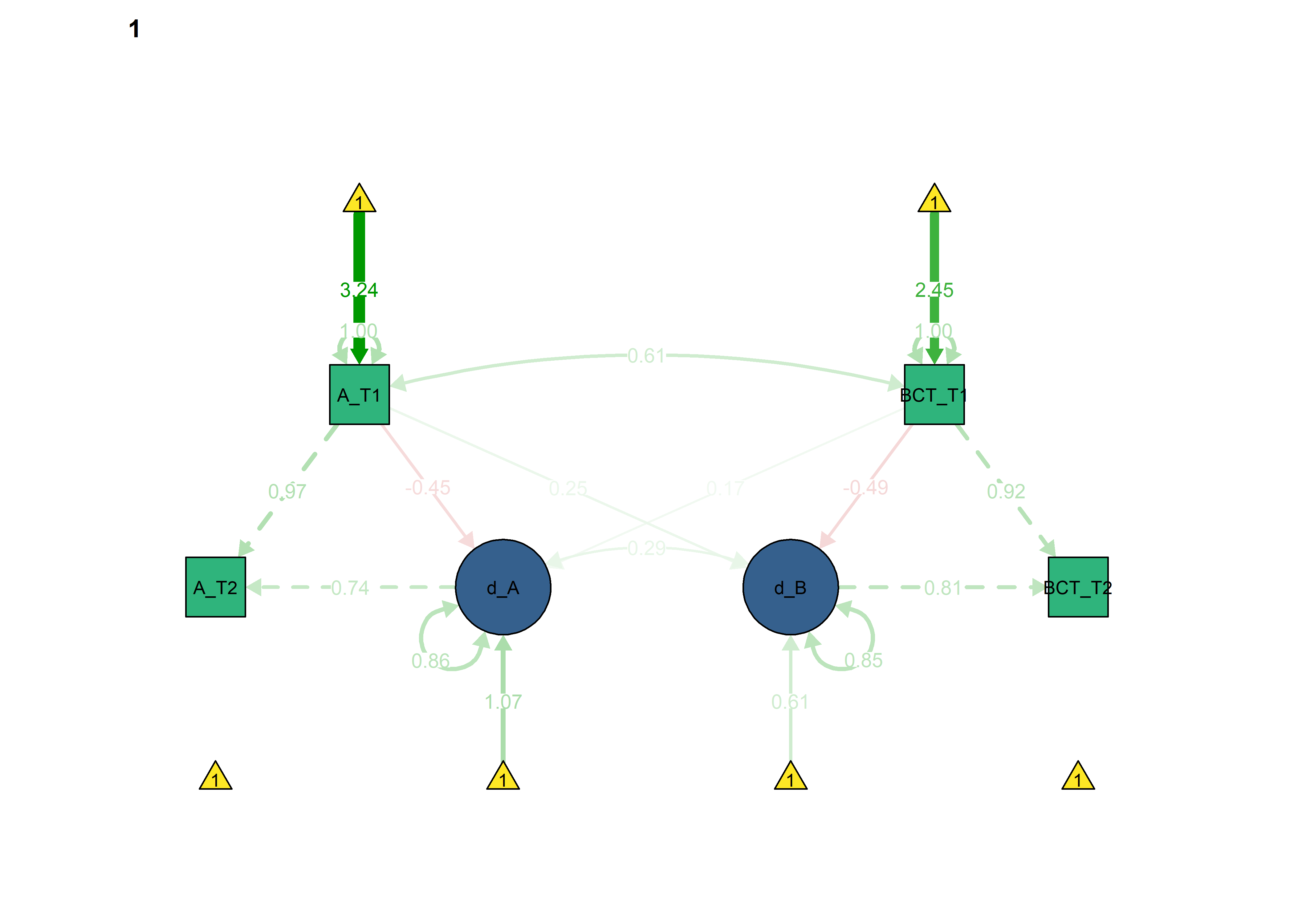

Constraints for the four educational tracks
Basic model
data_BLCS <- df %>% dplyr::select(
track,
Autonomous_T1 = PA_autonomous_T1,
Autonomous_T2 = PA_autonomous_T3,
frqbct_T1 = PA_frqbct_T1,
frqbct_T2 = PA_frqbct_T3,
agrbct_T1 = PA_agrbct_T1,
agrbct_T2 = PA_agrbct_T3) %>%
filter(track != "Other") %>%
rowwise() %>%
dplyr::mutate(BCTs_T1 = mean(c(frqbct_T1, agrbct_T1), na.rm = TRUE),
BCTs_T2 = mean(c(frqbct_T2, agrbct_T2), na.rm = TRUE)) %>%
dplyr::select(-contains("frq"), -contains("agr"))
#Fit the Bivariate Latent Change Score model to simulated data
BLCS <- '
Autonomous_T2 ~ 1 * Autonomous_T1 # This parameter regresses Autonomous_T2 perfectly on Autonomous_T1
d_Autonomous1 =~ 1 * Autonomous_T2 # This defines the latent change score factor as measured perfectly by scores on Autonomous_T2
d_Autonomous1 ~ 1 # This estimates the intercept of the change score
Autonomous_T1 ~ 1 # This constrains the intercept of Autonomous_T1 to be identical across intervention and control groups
Autonomous_T2 ~ 0 * 1 # This constrains the intercept of Autonomous_T2 to 0
BCTs_T2 ~ 1 * BCTs_T1 # This parameter regresses BCTs_T2 perfectly on BCTs_T1
d_BCTs1 =~ 1 * BCTs_T2 # This defines the latent change score factor as measured perfectly by scores on BCTs_T2
BCTs_T2 ~ 0 * 1 # This line constrains the intercept of BCTs_T2 to 0
BCTs_T2 ~~ 0 * BCTs_T2 # This fixes the variance of the BCTs_T1 to 0
d_Autonomous1 ~~ d_Autonomous1 # This estimates the variance of the change scores
Autonomous_T1 ~~ Autonomous_T1 # This estimates the variance of the Autonomous_T1
Autonomous_T2 ~~ 0 * Autonomous_T2 # This fixes the variance of the Autonomous_T2 to 0
d_BCTs1 ~ 1 # This estimates the intercept of the change score
BCTs_T1 ~ 1 # This estimates the intercept of BCTs_T1
d_BCTs1 ~~ d_BCTs1 # This estimates the variance of the change scores
BCTs_T1 ~~ BCTs_T1 # This estimates the variance of BCTs_T1
d_BCTs1 ~ Autonomous_T1 + BCTs_T1 # This estimates the autonomous to BCT coupling parameter and the BCT (T1) to BCT (T2) self-feedback
d_Autonomous1 ~ BCTs_T1 + Autonomous_T1 # This estimates the BCT to autonomous coupling parameter and the autonomous (T1) to autonomous (T2) self-feedback
Autonomous_T1 ~~ BCTs_T1 # This estimates the Autonomous_T1 BCTs_T1 covariance
d_Autonomous1 ~~ d_BCTs1 # This estimates the d_Autonomous and d_BCTs covariance
'
fitBLCS <- lavaan::lavaan(BLCS,
data = data_BLCS,
estimator = 'mlr',
fixed.x = FALSE,
group = "track",
missing = 'fiml')
## Warning in lav_data_full(data = data, group = group, cluster = cluster, : lavaan WARNING: some cases are empty and will be ignored:
## 79
lavaan::summary(fitBLCS, fit.measures = TRUE, standardized = TRUE, rsquare = TRUE)
## lavaan (0.5-23.1097) converged normally after 108 iterations
##
## Used Total
## Number of observations per group
## BA 281 282
## HRC 213 213
## IT 163 163
## Nur 402 402
##
## Number of missing patterns per group
## BA 7
## HRC 4
## IT 3
## Nur 6
##
## Estimator ML Robust
## Minimum Function Test Statistic 0.000 0.000
## Degrees of freedom 0 0
## Minimum Function Value 0.0000000000000
## Scaling correction factor NA
## for the Yuan-Bentler correction
##
## Chi-square for each group:
##
## BA 0.000 0.000
## HRC 0.000 0.000
## IT 0.000 0.000
## Nur 0.000 0.000
##
## Model test baseline model:
##
## Minimum Function Test Statistic 1618.796 1066.992
## Degrees of freedom 24 24
## P-value 0.000 0.000
##
## User model versus baseline model:
##
## Comparative Fit Index (CFI) 1.000 1.000
## Tucker-Lewis Index (TLI) 1.000 1.000
##
## Robust Comparative Fit Index (CFI) NA
## Robust Tucker-Lewis Index (TLI) NA
##
## Loglikelihood and Information Criteria:
##
## Loglikelihood user model (H0) -4894.474 -4894.474
## Loglikelihood unrestricted model (H1) -4894.474 -4894.474
##
## Number of free parameters 56 56
## Akaike (AIC) 9900.948 9900.948
## Bayesian (BIC) 10178.992 10178.992
## Sample-size adjusted Bayesian (BIC) 10001.127 10001.127
##
## Root Mean Square Error of Approximation:
##
## RMSEA 0.000 0.000
## 90 Percent Confidence Interval 0.000 0.000 0.000 0.000
## P-value RMSEA <= 0.05 NA NA
##
## Robust RMSEA 0.000
## 90 Percent Confidence Interval 0.000 0.000
##
## Standardized Root Mean Square Residual:
##
## SRMR 0.000 0.000
##
## Parameter Estimates:
##
## Information Observed
## Standard Errors Robust.huber.white
##
##
## Group 1 [BA]:
##
## Latent Variables:
## Estimate Std.Err z-value P(>|z|) Std.lv Std.all
## d_Autonomous1 =~
## Autonomous_T2 1.000 0.752 0.753
## d_BCTs1 =~
## BCTs_T2 1.000 1.047 0.876
##
## Regressions:
## Estimate Std.Err z-value P(>|z|) Std.lv Std.all
## Autonomous_T2 ~
## Autonomous_T1 1.000 1.000 0.982
## BCTs_T2 ~
## BCTs_T1 1.000 1.000 0.931
## d_BCTs1 ~
## Autonomous_T1 0.226 0.112 2.018 0.044 0.216 0.212
## BCTs_T1 -0.488 0.117 -4.165 0.000 -0.466 -0.519
## d_Autonomous1 ~
## BCTs_T1 0.056 0.079 0.707 0.479 0.075 0.083
## Autonomous_T1 -0.315 0.077 -4.107 0.000 -0.419 -0.411
##
## Covariances:
## Estimate Std.Err z-value P(>|z|) Std.lv Std.all
## Autonomous_T1 ~~
## BCTs_T1 0.674 0.070 9.634 0.000 0.674 0.618
## .d_Autonomous1 ~~
## .d_BCTs1 0.112 0.059 1.912 0.056 0.169 0.169
##
## Intercepts:
## Estimate Std.Err z-value P(>|z|) Std.lv Std.all
## .d_Autonomous1 0.935 0.187 4.993 0.000 1.243 1.243
## Autonomous_T1 3.618 0.059 61.845 0.000 3.618 3.690
## .Autonomous_T2 0.000 0.000 0.000
## .BCTs_T2 0.000 0.000 0.000
## .d_BCTs1 0.877 0.231 3.793 0.000 0.837 0.837
## BCTs_T1 3.099 0.067 46.459 0.000 3.099 2.783
##
## Variances:
## Estimate Std.Err z-value P(>|z|) Std.lv Std.all
## .BCTs_T2 0.000 0.000 0.000
## .d_Autonomous1 0.490 0.066 7.366 0.000 0.867 0.867
## Autonomous_T1 0.961 0.076 12.718 0.000 0.961 1.000
## .Autonomous_T2 0.000 0.000 0.000
## .d_BCTs1 0.901 0.095 9.494 0.000 0.821 0.821
## BCTs_T1 1.240 0.094 13.163 0.000 1.240 1.000
##
## R-Square:
## Estimate
## BCTs_T2 1.000
## d_Autonomous1 0.133
## Autonomous_T2 1.000
## d_BCTs1 0.179
##
##
## Group 2 [HRC]:
##
## Latent Variables:
## Estimate Std.Err z-value P(>|z|) Std.lv Std.all
## d_Autonomous1 =~
## Autonomous_T2 1.000 0.760 0.766
## d_BCTs1 =~
## BCTs_T2 1.000 0.972 0.804
##
## Regressions:
## Estimate Std.Err z-value P(>|z|) Std.lv Std.all
## Autonomous_T2 ~
## Autonomous_T1 1.000 1.000 1.069
## BCTs_T2 ~
## BCTs_T1 1.000 1.000 0.966
## d_BCTs1 ~
## Autonomous_T1 0.175 0.091 1.936 0.053 0.181 0.192
## BCTs_T1 -0.398 0.095 -4.184 0.000 -0.410 -0.478
## d_Autonomous1 ~
## BCTs_T1 0.134 0.058 2.304 0.021 0.177 0.206
## Autonomous_T1 -0.401 0.076 -5.252 0.000 -0.527 -0.559
##
## Covariances:
## Estimate Std.Err z-value P(>|z|) Std.lv Std.all
## Autonomous_T1 ~~
## BCTs_T1 0.678 0.090 7.514 0.000 0.678 0.547
## .d_Autonomous1 ~~
## .d_BCTs1 0.164 0.050 3.297 0.001 0.277 0.277
##
## Intercepts:
## Estimate Std.Err z-value P(>|z|) Std.lv Std.all
## .d_Autonomous1 1.087 0.218 4.989 0.000 1.430 1.430
## Autonomous_T1 3.413 0.073 46.889 0.000 3.413 3.217
## .Autonomous_T2 0.000 0.000 0.000
## .BCTs_T2 0.000 0.000 0.000
## .d_BCTs1 0.541 0.219 2.468 0.014 0.557 0.557
## BCTs_T1 2.843 0.080 35.504 0.000 2.843 2.435
##
## Variances:
## Estimate Std.Err z-value P(>|z|) Std.lv Std.all
## .BCTs_T2 0.000 0.000 0.000
## .d_Autonomous1 0.446 0.080 5.606 0.000 0.771 0.771
## Autonomous_T1 1.125 0.092 12.264 0.000 1.125 1.000
## .Autonomous_T2 0.000 0.000 0.000
## .d_BCTs1 0.788 0.097 8.096 0.000 0.835 0.835
## BCTs_T1 1.362 0.119 11.495 0.000 1.362 1.000
##
## R-Square:
## Estimate
## BCTs_T2 1.000
## d_Autonomous1 0.229
## Autonomous_T2 1.000
## d_BCTs1 0.165
##
##
## Group 3 [IT]:
##
## Latent Variables:
## Estimate Std.Err z-value P(>|z|) Std.lv Std.all
## d_Autonomous1 =~
## Autonomous_T2 1.000 0.677 0.610
## d_BCTs1 =~
## BCTs_T2 1.000 1.016 0.858
##
## Regressions:
## Estimate Std.Err z-value P(>|z|) Std.lv Std.all
## Autonomous_T2 ~
## Autonomous_T1 1.000 1.000 0.973
## BCTs_T2 ~
## BCTs_T1 1.000 1.000 0.932
## d_BCTs1 ~
## Autonomous_T1 0.335 0.096 3.483 0.000 0.330 0.356
## BCTs_T1 -0.581 0.104 -5.586 0.000 -0.571 -0.631
## d_Autonomous1 ~
## BCTs_T1 0.090 0.066 1.363 0.173 0.133 0.147
## Autonomous_T1 -0.233 0.074 -3.137 0.002 -0.344 -0.372
##
## Covariances:
## Estimate Std.Err z-value P(>|z|) Std.lv Std.all
## Autonomous_T1 ~~
## BCTs_T1 0.847 0.098 8.682 0.000 0.847 0.710
## .d_Autonomous1 ~~
## .d_BCTs1 0.201 0.061 3.301 0.001 0.343 0.343
##
## Intercepts:
## Estimate Std.Err z-value P(>|z|) Std.lv Std.all
## .d_Autonomous1 0.508 0.150 3.380 0.001 0.751 0.751
## Autonomous_T1 2.875 0.085 33.951 0.000 2.875 2.662
## .Autonomous_T2 0.000 0.000 0.000
## .BCTs_T2 0.000 0.000 0.000
## .d_BCTs1 0.452 0.193 2.344 0.019 0.445 0.445
## BCTs_T1 2.363 0.087 27.263 0.000 2.363 2.140
##
## Variances:
## Estimate Std.Err z-value P(>|z|) Std.lv Std.all
## .BCTs_T2 0.000 0.000 0.000
## .d_Autonomous1 0.421 0.060 7.059 0.000 0.918 0.918
## Autonomous_T1 1.166 0.099 11.724 0.000 1.166 1.000
## .Autonomous_T2 0.000 0.000 0.000
## .d_BCTs1 0.821 0.111 7.388 0.000 0.794 0.794
## BCTs_T1 1.220 0.128 9.497 0.000 1.220 1.000
##
## R-Square:
## Estimate
## BCTs_T2 1.000
## d_Autonomous1 0.082
## Autonomous_T2 1.000
## d_BCTs1 0.206
##
##
## Group 4 [Nur]:
##
## Latent Variables:
## Estimate Std.Err z-value P(>|z|) Std.lv Std.all
## d_Autonomous1 =~
## Autonomous_T2 1.000 0.768 0.765
## d_BCTs1 =~
## BCTs_T2 1.000 1.032 0.902
##
## Regressions:
## Estimate Std.Err z-value P(>|z|) Std.lv Std.all
## Autonomous_T2 ~
## Autonomous_T1 1.000 1.000 1.018
## BCTs_T2 ~
## BCTs_T1 1.000 1.000 0.969
## d_BCTs1 ~
## Autonomous_T1 0.190 0.064 2.973 0.003 0.184 0.188
## BCTs_T1 -0.500 0.061 -8.251 0.000 -0.485 -0.537
## d_Autonomous1 ~
## BCTs_T1 0.139 0.048 2.870 0.004 0.181 0.200
## Autonomous_T1 -0.385 0.056 -6.929 0.000 -0.502 -0.512
##
## Covariances:
## Estimate Std.Err z-value P(>|z|) Std.lv Std.all
## Autonomous_T1 ~~
## BCTs_T1 0.640 0.055 11.558 0.000 0.640 0.566
## .d_Autonomous1 ~~
## .d_BCTs1 0.139 0.040 3.486 0.000 0.219 0.219
##
## Intercepts:
## Estimate Std.Err z-value P(>|z|) Std.lv Std.all
## .d_Autonomous1 1.022 0.145 7.038 0.000 1.332 1.332
## Autonomous_T1 3.470 0.051 68.060 0.000 3.470 3.399
## .Autonomous_T2 0.000 0.000 0.000
## .BCTs_T2 0.000 0.000 0.000
## .d_BCTs1 0.929 0.171 5.430 0.000 0.900 0.900
## BCTs_T1 2.779 0.055 50.156 0.000 2.779 2.508
##
## Variances:
## Estimate Std.Err z-value P(>|z|) Std.lv Std.all
## .BCTs_T2 0.000 0.000 0.000
## .d_Autonomous1 0.479 0.047 10.092 0.000 0.814 0.814
## Autonomous_T1 1.042 0.060 17.231 0.000 1.042 1.000
## .Autonomous_T2 0.000 0.000 0.000
## .d_BCTs1 0.841 0.065 13.029 0.000 0.790 0.790
## BCTs_T1 1.228 0.076 16.169 0.000 1.228 1.000
##
## R-Square:
## Estimate
## BCTs_T2 1.000
## d_Autonomous1 0.186
## Autonomous_T2 1.000
## d_BCTs1 0.210
semPlot::semPaths(fitBLCS,
what = "std",
ask = FALSE,
label.cex = .6,
label.scale = FALSE,
edge.label.cex = 0.75,
layout = "tree2",
intercepts = TRUE,
color = list(lat = viridis::viridis(3, begin = 0.3)[1],
man = viridis::viridis(3, begin = 0.3)[2],
int = viridis::viridis(3, begin = 0.3)[3]))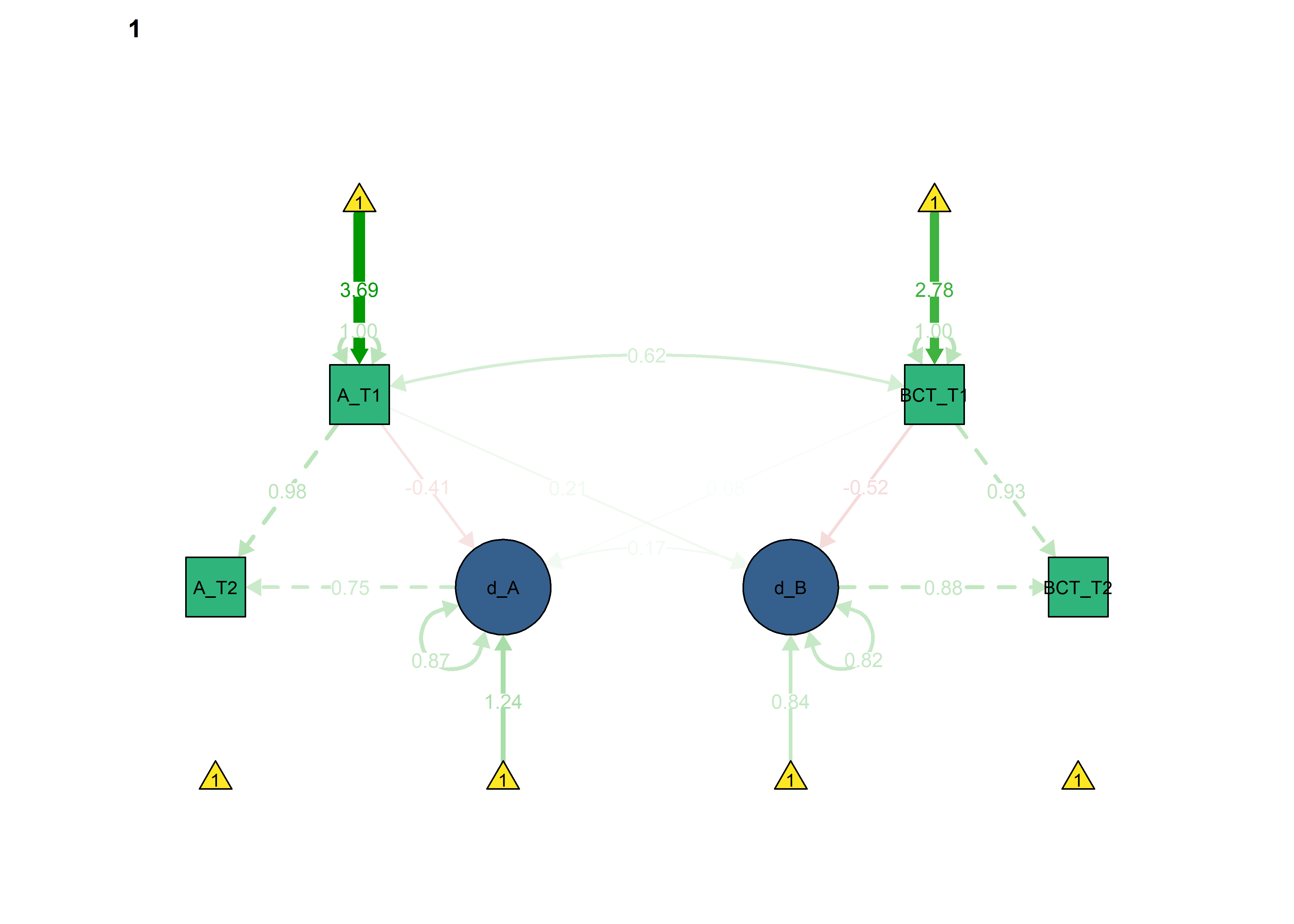
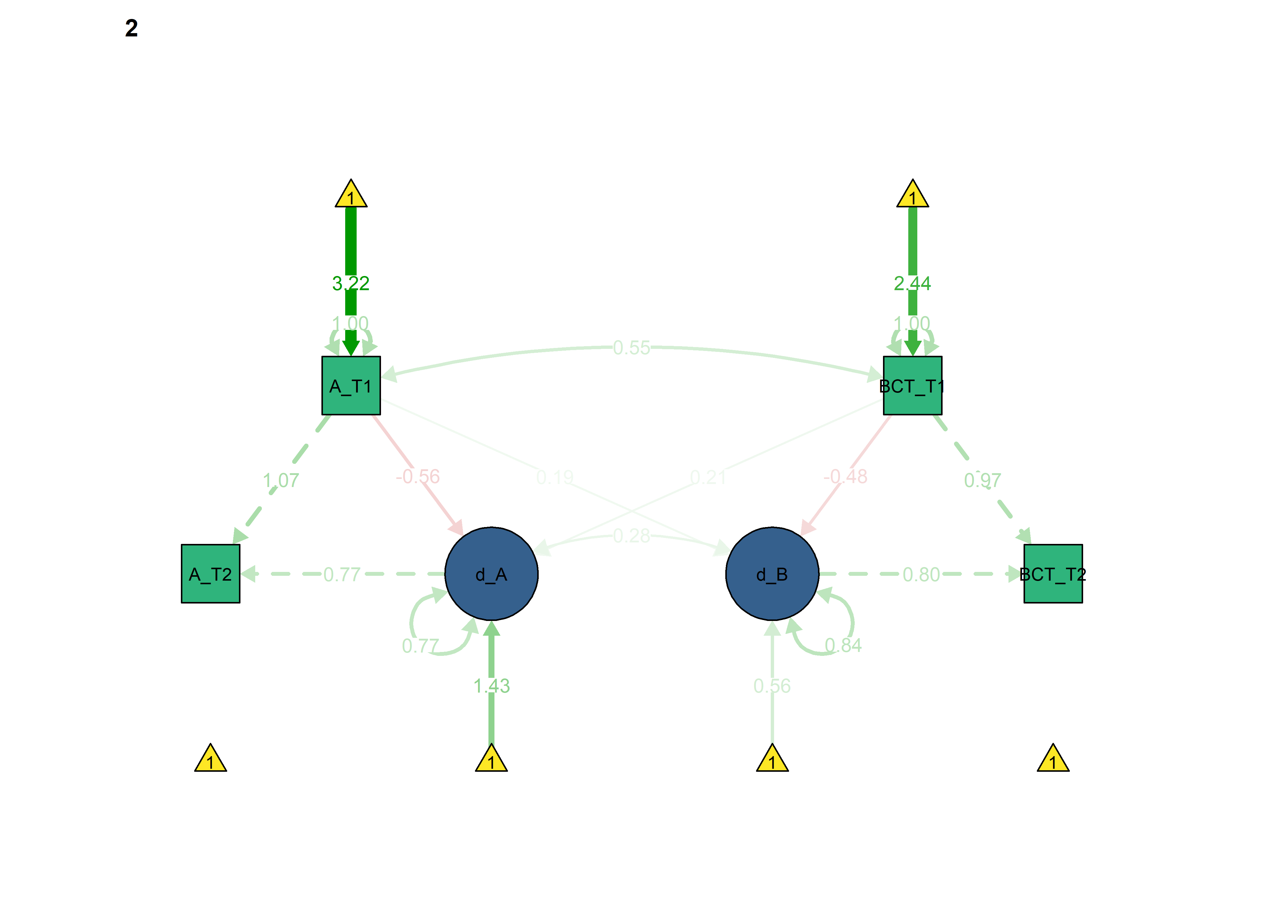
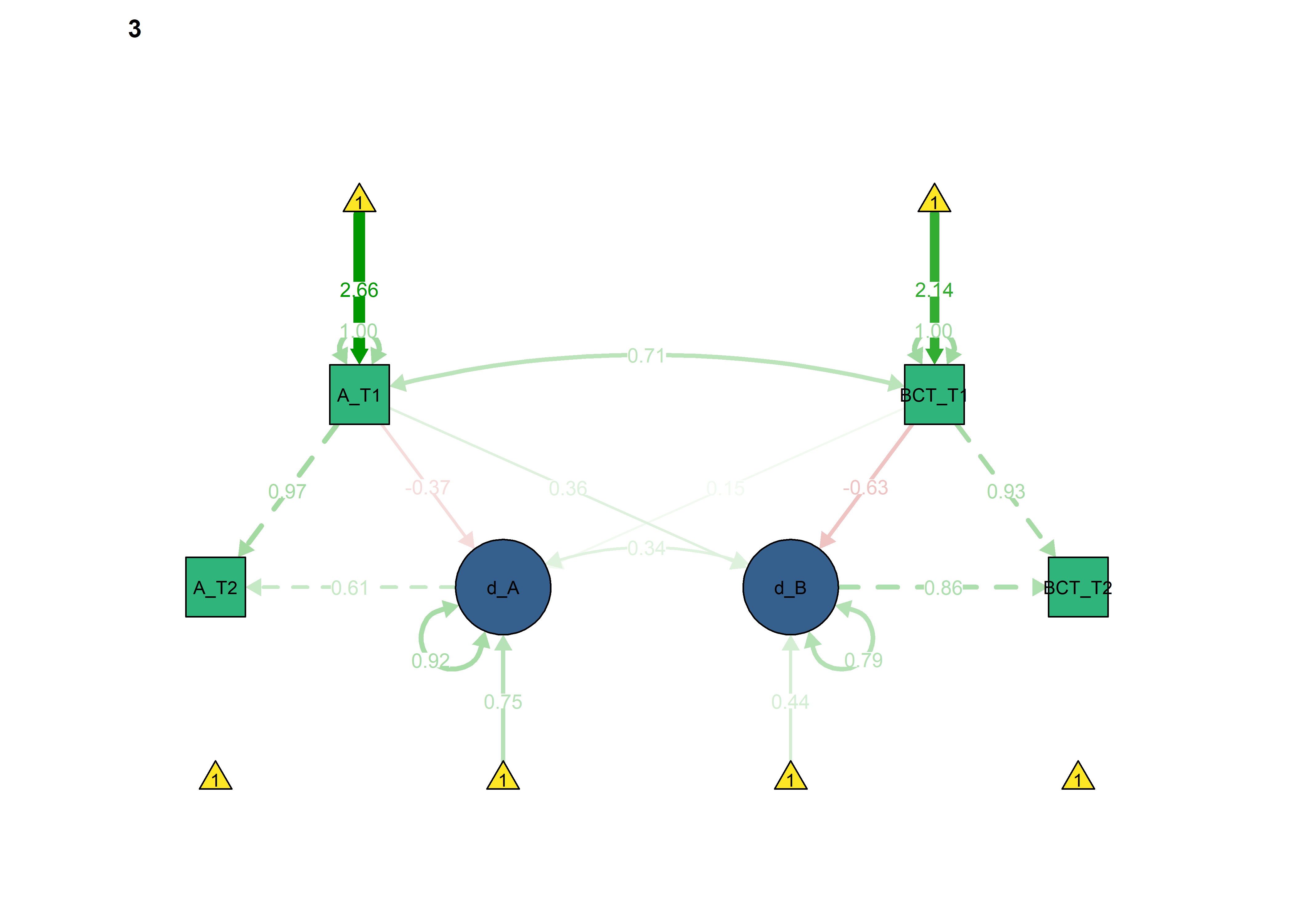
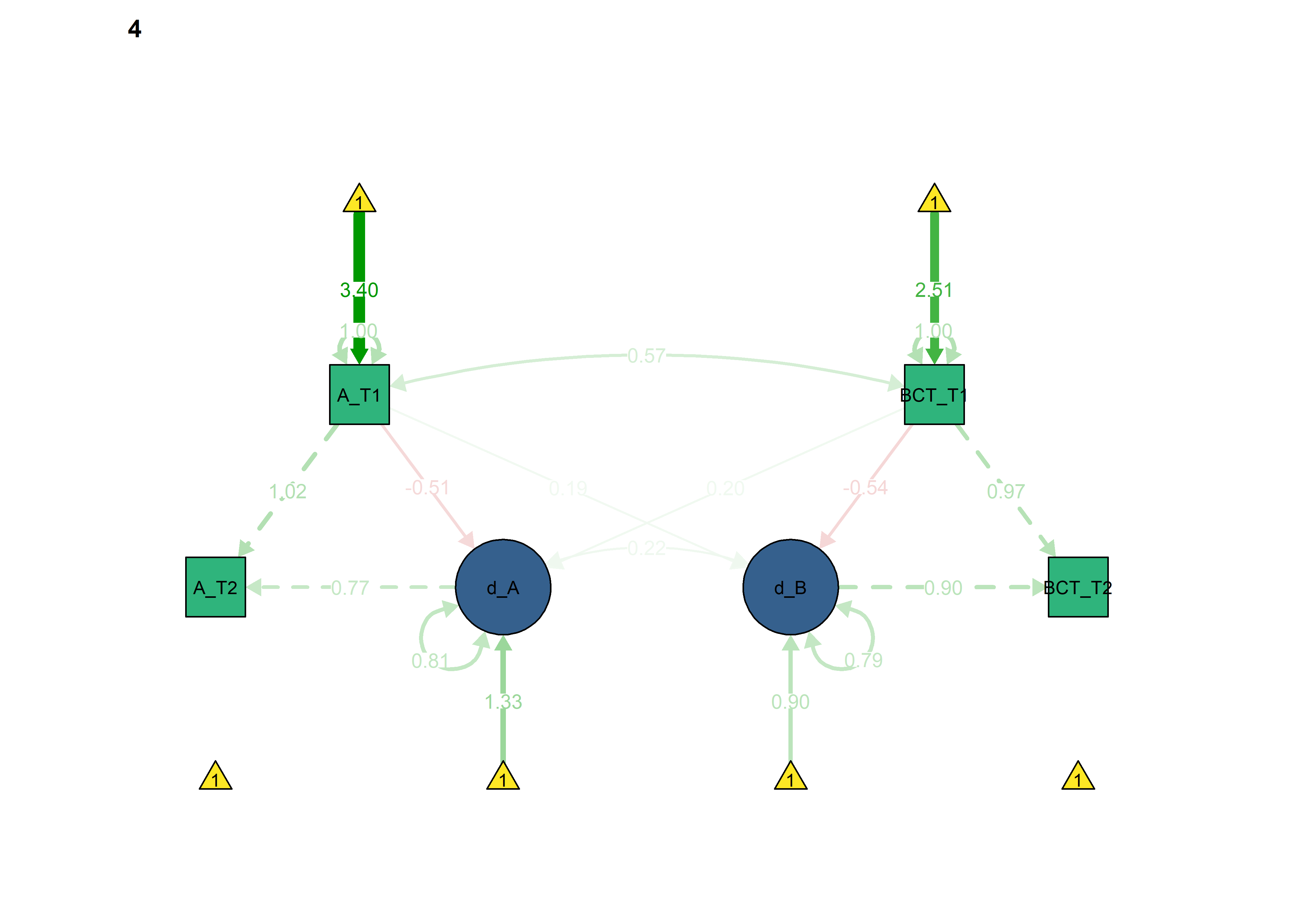
Expected constraints model
data_BLCS <- df %>% dplyr::select(
track,
Autonomous_T1 = PA_autonomous_T1,
Autonomous_T2 = PA_autonomous_T3,
frqbct_T1 = PA_frqbct_T1,
frqbct_T2 = PA_frqbct_T3,
agrbct_T1 = PA_agrbct_T1,
agrbct_T2 = PA_agrbct_T3) %>%
filter(track != "Other") %>%
rowwise() %>%
dplyr::mutate(BCTs_T1 = mean(c(frqbct_T1, agrbct_T1), na.rm = TRUE),
BCTs_T2 = mean(c(frqbct_T2, agrbct_T2), na.rm = TRUE)) %>%
dplyr::select(-contains("frq"), -contains("agr"))
#Fit the Bivariate Latent Change Score model to simulated data
BLCS_constrained <- '
Autonomous_T2 ~ 1 * Autonomous_T1 # This parameter regresses Autonomous_T2 perfectly on Autonomous_T1
d_Autonomous1 =~ 1 * Autonomous_T2 # This defines the latent change score factor as measured perfectly by scores on Autonomous_T2
d_Autonomous1 ~ 1 # This estimates the intercept of the change score
Autonomous_T1 ~ c(autint, autint, autint, autint) * 1 # This constrains the intercept of Autonomous_T1 to be identical across intervention and control groups
Autonomous_T2 ~ 0 * 1 # This constrains the intercept of Autonomous_T2 to 0
BCTs_T2 ~ 1 * BCTs_T1 # This parameter regresses BCTs_T2 perfectly on BCTs_T1
d_BCTs1 =~ 1 * BCTs_T2 # This defines the latent change score factor as measured perfectly by scores on BCTs_T2
BCTs_T2 ~ 0 * 1 # This line constrains the intercept of BCTs_T2 to 0
BCTs_T2 ~~ 0 * BCTs_T2 # This fixes the variance of the BCTs_T1 to 0
d_Autonomous1 ~~ d_Autonomous1 # This estimates the variance of the change scores
Autonomous_T1 ~~ c(autvar, autvar, autvar, autvar) * Autonomous_T1 # This estimates the variance of the Autonomous_T1
Autonomous_T2 ~~ 0 * Autonomous_T2 # This fixes the variance of the Autonomous_T2 to 0
d_BCTs1 ~ 1 # This estimates the intercept of the change score
BCTs_T1 ~ c(bctint, bctint, bctint, bctint) * 1 # This estimates the intercept of BCTs_T1
d_BCTs1 ~~ d_BCTs1 # This estimates the variance of the change scores
BCTs_T1 ~~ c(bctvar, bctvar, bctvar, bctvar) * BCTs_T1 # This estimates the variance of BCTs_T1
d_BCTs1 ~ Autonomous_T1 + BCTs_T1 # This estimates the autonomous to BCT coupling parameter and the BCT (T1) to BCT (T2) self-feedback
d_Autonomous1 ~ BCTs_T1 + Autonomous_T1 # This estimates the BCT to autonomous coupling parameter and the autonomous (T1) to autonomous (T2) self-feedback
Autonomous_T1 ~~ c(autbct_cov, autbct_cov, autbct_cov, autbct_cov) * BCTs_T1 # This estimates the Autonomous_T1 BCTs_T1 covariance
d_Autonomous1 ~~ d_BCTs1 # This estimates the d_Autonomous and d_BCTs covariance
'
fitBLCS_constrained <- lavaan::lavaan(BLCS_constrained,
data = data_BLCS,
estimator = 'mlr',
fixed.x = FALSE,
group = "track",
missing = 'fiml')
## Warning in lav_data_full(data = data, group = group, cluster = cluster, : lavaan WARNING: some cases are empty and will be ignored:
## 79
lavaan::summary(fitBLCS_constrained, fit.measures = TRUE, standardized = TRUE, rsquare = TRUE)
## lavaan (0.5-23.1097) converged normally after 91 iterations
##
## Used Total
## Number of observations per group
## BA 281 282
## HRC 213 213
## IT 163 163
## Nur 402 402
##
## Number of missing patterns per group
## BA 7
## HRC 4
## IT 3
## Nur 6
##
## Estimator ML Robust
## Minimum Function Test Statistic 83.779 88.903
## Degrees of freedom 15 15
## P-value (Chi-square) 0.000 0.000
## Scaling correction factor 0.942
## for the Yuan-Bentler correction
##
## Chi-square for each group:
##
## BA 22.423 23.794
## HRC 3.996 4.241
## IT 50.823 53.931
## Nur 6.536 6.936
##
## Model test baseline model:
##
## Minimum Function Test Statistic 1618.796 1066.992
## Degrees of freedom 24 24
## P-value 0.000 0.000
##
## User model versus baseline model:
##
## Comparative Fit Index (CFI) 0.957 0.929
## Tucker-Lewis Index (TLI) 0.931 0.887
##
## Robust Comparative Fit Index (CFI) 0.956
## Robust Tucker-Lewis Index (TLI) 0.930
##
## Loglikelihood and Information Criteria:
##
## Loglikelihood user model (H0) -4936.363 -4936.363
## Scaling correction factor 0.908
## for the MLR correction
## Loglikelihood unrestricted model (H1) -4894.474 -4894.474
## Scaling correction factor 1.161
## for the MLR correction
##
## Number of free parameters 41 41
## Akaike (AIC) 9954.727 9954.727
## Bayesian (BIC) 10158.295 10158.295
## Sample-size adjusted Bayesian (BIC) 10028.072 10028.072
##
## Root Mean Square Error of Approximation:
##
## RMSEA 0.132 0.136
## 90 Percent Confidence Interval 0.105 0.160 0.109 0.165
## P-value RMSEA <= 0.05 0.000 0.000
##
## Robust RMSEA 0.132
## 90 Percent Confidence Interval 0.107 0.160
##
## Standardized Root Mean Square Residual:
##
## SRMR 0.093 0.093
##
## Parameter Estimates:
##
## Information Observed
## Standard Errors Robust.huber.white
##
##
## Group 1 [BA]:
##
## Latent Variables:
## Estimate Std.Err z-value P(>|z|) Std.lv Std.all
## d_Autonomous1 =~
## Autonomous_T2 1.000 0.760 0.734
## d_BCTs1 =~
## BCTs_T2 1.000 1.052 0.867
##
## Regressions:
## Estimate Std.Err z-value P(>|z|) Std.lv Std.all
## Autonomous_T2 ~
## Autonomous_T1 1.000 1.000 1.018
## BCTs_T2 ~
## BCTs_T1 1.000 1.000 0.944
## d_BCTs1 ~
## Autonomous_T1 0.226 0.112 2.016 0.044 0.215 0.226
## BCTs_T1 -0.488 0.117 -4.167 0.000 -0.464 -0.531
## d_Autonomous1 ~
## BCTs_T1 0.055 0.079 0.702 0.483 0.073 0.084
## Autonomous_T1 -0.314 0.077 -4.107 0.000 -0.414 -0.436
##
## Covariances:
## Estimate Std.Err z-value P(>|z|) Std.lv Std.all
## Autonomous_T1 ~~
## BCTs_T1 (atb_) 0.740 0.038 19.726 0.000 0.740 0.613
## .d_Autonomous1 ~~
## .d_BCTs1 0.112 0.059 1.917 0.055 0.169 0.169
##
## Intercepts:
## Estimate Std.Err z-value P(>|z|) Std.lv Std.all
## .d_Atnm1 0.936 0.187 4.993 0.000 1.230 1.230
## Atnm_T1 (atnt) 3.407 0.032 104.949 0.000 3.407 3.228
## .Atnm_T2 0.000 0.000 0.000
## .BCTs_T2 0.000 0.000 0.000
## .d_BCTs1 0.878 0.231 3.799 0.000 0.834 0.834
## BCTs_T1 (bctn) 2.813 0.035 79.751 0.000 2.813 2.457
##
## Variances:
## Estimate Std.Err z-value P(>|z|) Std.lv Std.all
## .BCTs_T2 0.000 0.000 0.000
## .d_Atnm1 0.490 0.067 7.357 0.000 0.847 0.847
## Atnm_T1 (atvr) 1.113 0.040 27.929 0.000 1.113 1.000
## .Atnm_T2 0.000 0.000 0.000
## .d_BCTs1 0.900 0.095 9.493 0.000 0.814 0.814
## BCTs_T1 (bctv) 1.310 0.050 26.235 0.000 1.310 1.000
##
## R-Square:
## Estimate
## BCTs_T2 1.000
## d_Autonomous1 0.153
## Autonomous_T2 1.000
## d_BCTs1 0.186
##
##
## Group 2 [HRC]:
##
## Latent Variables:
## Estimate Std.Err z-value P(>|z|) Std.lv Std.all
## d_Autonomous1 =~
## Autonomous_T2 1.000 0.754 0.758
## d_BCTs1 =~
## BCTs_T2 1.000 0.963 0.798
##
## Regressions:
## Estimate Std.Err z-value P(>|z|) Std.lv Std.all
## Autonomous_T2 ~
## Autonomous_T1 1.000 1.000 1.061
## BCTs_T2 ~
## BCTs_T1 1.000 1.000 0.949
## d_BCTs1 ~
## Autonomous_T1 0.175 0.091 1.935 0.053 0.182 0.192
## BCTs_T1 -0.398 0.095 -4.182 0.000 -0.413 -0.473
## d_Autonomous1 ~
## BCTs_T1 0.134 0.058 2.303 0.021 0.178 0.204
## Autonomous_T1 -0.401 0.076 -5.251 0.000 -0.531 -0.561
##
## Covariances:
## Estimate Std.Err z-value P(>|z|) Std.lv Std.all
## Autonomous_T1 ~~
## BCTs_T1 (atb_) 0.740 0.038 19.726 0.000 0.740 0.613
## .d_Autonomous1 ~~
## .d_BCTs1 0.164 0.050 3.297 0.001 0.277 0.277
##
## Intercepts:
## Estimate Std.Err z-value P(>|z|) Std.lv Std.all
## .d_Atnm1 1.087 0.218 4.989 0.000 1.442 1.442
## Atnm_T1 (atnt) 3.407 0.032 104.949 0.000 3.407 3.228
## .Atnm_T2 0.000 0.000 0.000
## .BCTs_T2 0.000 0.000 0.000
## .d_BCTs1 0.541 0.219 2.470 0.014 0.562 0.562
## BCTs_T1 (bctn) 2.813 0.035 79.751 0.000 2.813 2.457
##
## Variances:
## Estimate Std.Err z-value P(>|z|) Std.lv Std.all
## .BCTs_T2 0.000 0.000 0.000
## .d_Atnm1 0.446 0.080 5.606 0.000 0.784 0.784
## Atnm_T1 (atvr) 1.113 0.040 27.929 0.000 1.113 1.000
## .Atnm_T2 0.000 0.000 0.000
## .d_BCTs1 0.788 0.097 8.094 0.000 0.851 0.851
## BCTs_T1 (bctv) 1.310 0.050 26.235 0.000 1.310 1.000
##
## R-Square:
## Estimate
## BCTs_T2 1.000
## d_Autonomous1 0.216
## Autonomous_T2 1.000
## d_BCTs1 0.149
##
##
## Group 3 [IT]:
##
## Latent Variables:
## Estimate Std.Err z-value P(>|z|) Std.lv Std.all
## d_Autonomous1 =~
## Autonomous_T2 1.000 0.679 0.623
## d_BCTs1 =~
## BCTs_T2 1.000 1.049 0.892
##
## Regressions:
## Estimate Std.Err z-value P(>|z|) Std.lv Std.all
## Autonomous_T2 ~
## Autonomous_T1 1.000 1.000 0.968
## BCTs_T2 ~
## BCTs_T1 1.000 1.000 0.973
## d_BCTs1 ~
## Autonomous_T1 0.335 0.096 3.488 0.000 0.320 0.337
## BCTs_T1 -0.581 0.104 -5.596 0.000 -0.554 -0.634
## d_Autonomous1 ~
## BCTs_T1 0.090 0.066 1.368 0.171 0.133 0.152
## Autonomous_T1 -0.234 0.074 -3.141 0.002 -0.344 -0.363
##
## Covariances:
## Estimate Std.Err z-value P(>|z|) Std.lv Std.all
## Autonomous_T1 ~~
## BCTs_T1 (atb_) 0.740 0.038 19.726 0.000 0.740 0.613
## .d_Autonomous1 ~~
## .d_BCTs1 0.201 0.061 3.302 0.001 0.343 0.343
##
## Intercepts:
## Estimate Std.Err z-value P(>|z|) Std.lv Std.all
## .d_Atnm1 0.508 0.150 3.378 0.001 0.748 0.748
## Atnm_T1 (atnt) 3.407 0.032 104.949 0.000 3.407 3.228
## .Atnm_T2 0.000 0.000 0.000
## .BCTs_T2 0.000 0.000 0.000
## .d_BCTs1 0.452 0.193 2.345 0.019 0.431 0.431
## BCTs_T1 (bctn) 2.813 0.035 79.751 0.000 2.813 2.457
##
## Variances:
## Estimate Std.Err z-value P(>|z|) Std.lv Std.all
## .BCTs_T2 0.000 0.000 0.000
## .d_Atnm1 0.421 0.060 7.060 0.000 0.913 0.913
## Atnm_T1 (atvr) 1.113 0.040 27.929 0.000 1.113 1.000
## .Atnm_T2 0.000 0.000 0.000
## .d_BCTs1 0.821 0.111 7.390 0.000 0.746 0.746
## BCTs_T1 (bctv) 1.310 0.050 26.235 0.000 1.310 1.000
##
## R-Square:
## Estimate
## BCTs_T2 1.000
## d_Autonomous1 0.087
## Autonomous_T2 1.000
## d_BCTs1 0.254
##
##
## Group 4 [Nur]:
##
## Latent Variables:
## Estimate Std.Err z-value P(>|z|) Std.lv Std.all
## d_Autonomous1 =~
## Autonomous_T2 1.000 0.768 0.749
## d_BCTs1 =~
## BCTs_T2 1.000 1.034 0.890
##
## Regressions:
## Estimate Std.Err z-value P(>|z|) Std.lv Std.all
## Autonomous_T2 ~
## Autonomous_T1 1.000 1.000 1.029
## BCTs_T2 ~
## BCTs_T1 1.000 1.000 0.985
## d_BCTs1 ~
## Autonomous_T1 0.190 0.064 2.970 0.003 0.184 0.194
## BCTs_T1 -0.500 0.061 -8.250 0.000 -0.484 -0.554
## d_Autonomous1 ~
## BCTs_T1 0.139 0.048 2.874 0.004 0.181 0.207
## Autonomous_T1 -0.385 0.056 -6.932 0.000 -0.501 -0.529
##
## Covariances:
## Estimate Std.Err z-value P(>|z|) Std.lv Std.all
## Autonomous_T1 ~~
## BCTs_T1 (atb_) 0.740 0.038 19.726 0.000 0.740 0.613
## .d_Autonomous1 ~~
## .d_BCTs1 0.139 0.040 3.485 0.000 0.219 0.219
##
## Intercepts:
## Estimate Std.Err z-value P(>|z|) Std.lv Std.all
## .d_Atnm1 1.022 0.145 7.039 0.000 1.330 1.330
## Atnm_T1 (atnt) 3.407 0.032 104.949 0.000 3.407 3.228
## .Atnm_T2 0.000 0.000 0.000
## .BCTs_T2 0.000 0.000 0.000
## .d_BCTs1 0.929 0.171 5.431 0.000 0.899 0.899
## BCTs_T1 (bctn) 2.813 0.035 79.751 0.000 2.813 2.457
##
## Variances:
## Estimate Std.Err z-value P(>|z|) Std.lv Std.all
## .BCTs_T2 0.000 0.000 0.000
## .d_Atnm1 0.479 0.047 10.091 0.000 0.812 0.812
## Atnm_T1 (atvr) 1.113 0.040 27.929 0.000 1.113 1.000
## .Atnm_T2 0.000 0.000 0.000
## .d_BCTs1 0.842 0.065 13.028 0.000 0.787 0.787
## BCTs_T1 (bctv) 1.310 0.050 26.235 0.000 1.310 1.000
##
## R-Square:
## Estimate
## BCTs_T2 1.000
## d_Autonomous1 0.188
## Autonomous_T2 1.000
## d_BCTs1 0.213
lavaan::anova(fitBLCS, fitBLCS_constrained)
semPlot::semPaths(fitBLCS_constrained,
                  what = "std",
                  ask = FALSE,
                  label.cex = .6,
                  label.scale = FALSE,
                  edge.label.cex = 0.75,
                  layout = "tree2",
                  intercepts = TRUE,
                  color = list(lat = viridis::viridis(3, begin = 0.3)[1],
                               man = viridis::viridis(3, begin = 0.3)[2],
                               int = viridis::viridis(3, begin = 0.3)[3]))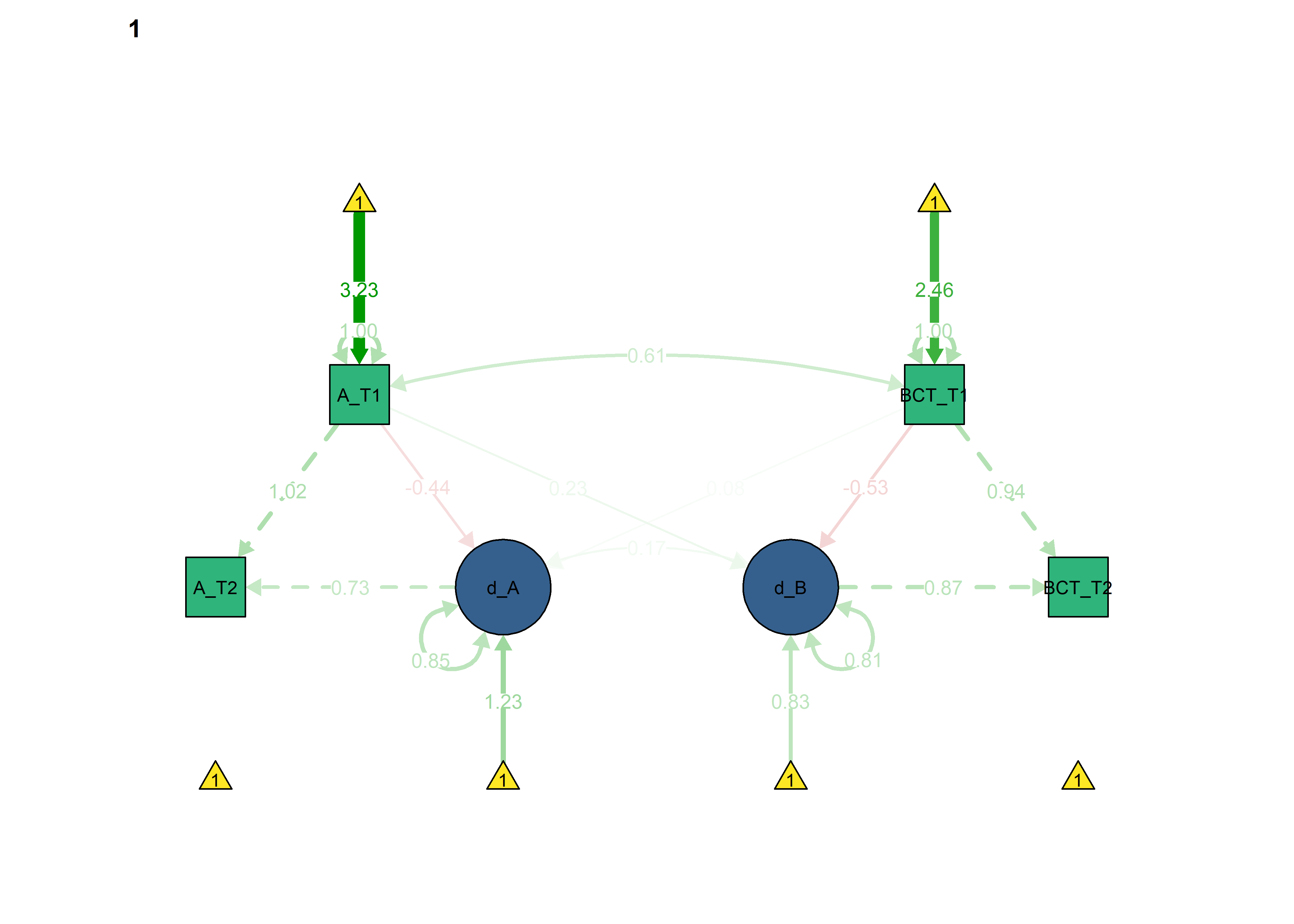
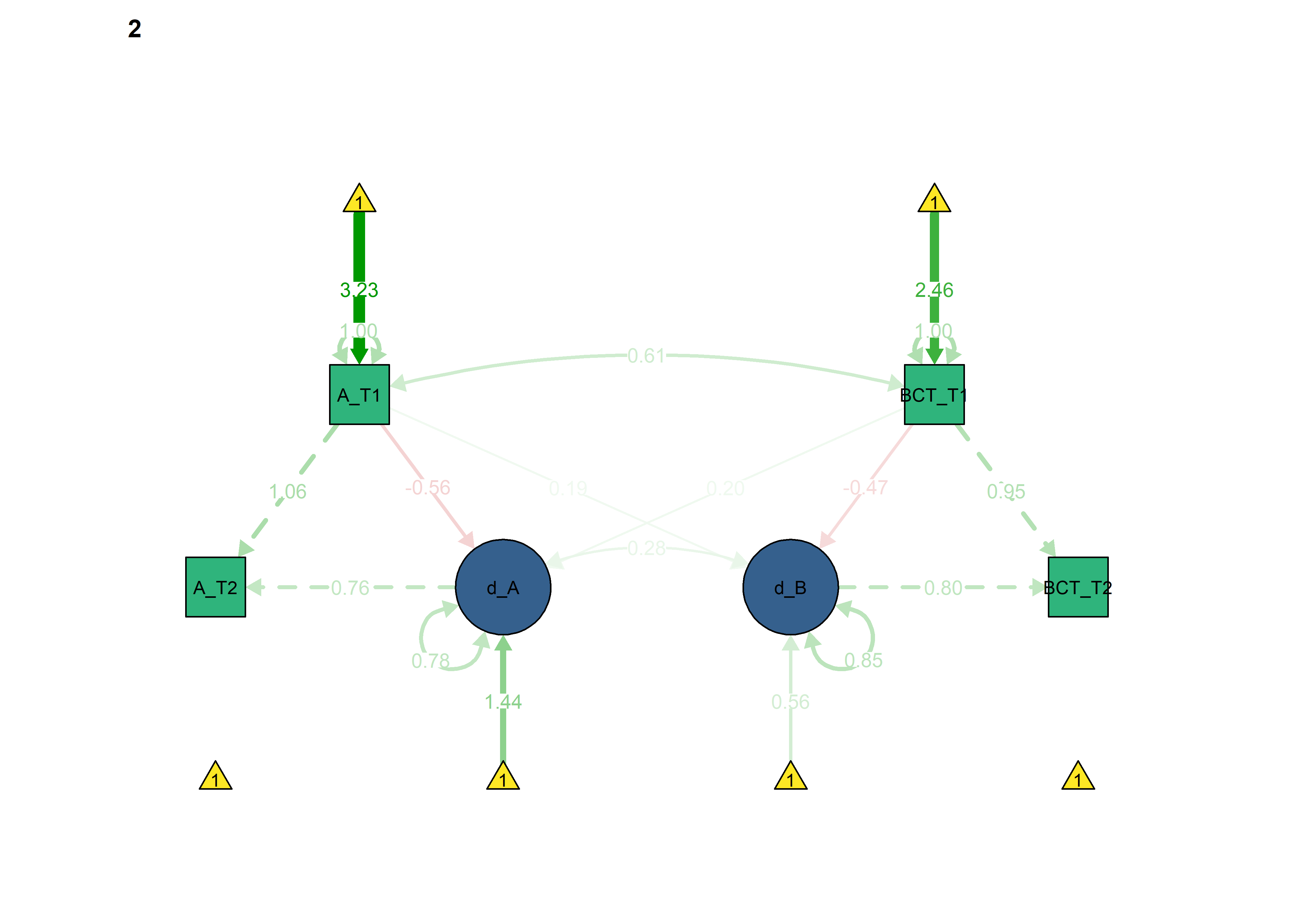


Turns out, that the model fits significantly better with
All constraints
data_BLCS <- df %>% dplyr::select(
track,
Autonomous_T1 = PA_autonomous_T1,
Autonomous_T2 = PA_autonomous_T3,
frqbct_T1 = PA_frqbct_T1,
frqbct_T2 = PA_frqbct_T3,
agrbct_T1 = PA_agrbct_T1,
agrbct_T2 = PA_agrbct_T3) %>%
filter(track != "Other") %>%
rowwise() %>%
dplyr::mutate(BCTs_T1 = mean(c(frqbct_T1, agrbct_T1), na.rm = TRUE),
BCTs_T2 = mean(c(frqbct_T2, agrbct_T2), na.rm = TRUE)) %>%
dplyr::select(-contains("frq"), -contains("agr"))
#Fit the Bivariate Latent Change Score model to simulated data
BLCS_allConstraints <- '
Autonomous_T2 ~ 1 * Autonomous_T1 # This parameter regresses Autonomous_T2 perfectly on Autonomous_T1
d_Autonomous1 =~ 1 * Autonomous_T2 # This defines the latent change score factor as measured perfectly by scores on Autonomous_T2
d_Autonomous1 ~ c(d_autint, d_autint, d_autint, d_autint) * 1 # This estimates the intercept of the change score
Autonomous_T1 ~ c(autint, autint, autint, autint) * 1 # This constrains the intercept of Autonomous_T1 to be identical across intervention and control groups
Autonomous_T2 ~ 0 * 1 # This constrains the intercept of Autonomous_T2 to 0
BCTs_T2 ~ 1 * BCTs_T1 # This parameter regresses BCTs_T2 perfectly on BCTs_T1
d_BCTs1 =~ 1 * BCTs_T2 # This defines the latent change score factor as measured perfectly by scores on BCTs_T2
BCTs_T2 ~ 0 * 1 # This line constrains the intercept of BCTs_T2 to 0
BCTs_T2 ~~ 0 * BCTs_T2 # This fixes the variance of the BCTs_T1 to 0
d_Autonomous1 ~~ d_Autonomous1 # This estimates the variance of the change scores
Autonomous_T1 ~~ c(autvar, autvar, autvar, autvar) * Autonomous_T1 # This estimates the variance of the Autonomous_T1
Autonomous_T2 ~~ 0 * Autonomous_T2 # This fixes the variance of the Autonomous_T2 to 0
d_BCTs1 ~ c(d_bctint, d_bctint, d_bctint, d_bctint) * 1 # This estimates the intercept of the change score
BCTs_T1 ~ c(bctint, bctint, bctint, bctint) * 1 # This estimates the intercept of BCTs_T1
d_BCTs1 ~~ d_BCTs1 # This estimates the variance of the change scores
BCTs_T1 ~~ c(bctvar, bctvar, bctvar, bctvar) * BCTs_T1 # This estimates the variance of BCTs_T1
d_BCTs1 ~ c(d_autbct, d_autbct, d_autbct, d_autbct) * Autonomous_T1 + BCTs_T1 # This estimates the autonomous to BCT coupling parameter and the BCT (T1) to BCT (T2) self-feedback
d_Autonomous1 ~ c(d_bctaut, d_bctaut, d_bctaut, d_bctaut) * BCTs_T1 + Autonomous_T1 # This estimates the BCT to autonomous coupling parameter and the autonomous (T1) to autonomous (T2) self-feedback
Autonomous_T1 ~~ c(autbct_cov, autbct_cov, autbct_cov, autbct_cov) * BCTs_T1 # This estimates the Autonomous_T1 BCTs_T1 covariance
d_Autonomous1 ~~ d_BCTs1 # This estimates the d_Autonomous and d_BCTs covariance
'
fitBLCS_allConstraints <- lavaan::lavaan(BLCS_allConstraints,
data = data_BLCS,
estimator = 'mlr',
fixed.x = FALSE,
group = "track",
missing = 'fiml')
## Warning in lav_data_full(data = data, group = group, cluster = cluster, : lavaan WARNING: some cases are empty and will be ignored:
## 79
lavaan::summary(fitBLCS_allConstraints, fit.measures = TRUE, standardized = TRUE, rsquare = TRUE)
## lavaan (0.5-23.1097) converged normally after 61 iterations
##
## Used Total
## Number of observations per group
## BA 281 282
## HRC 213 213
## IT 163 163
## Nur 402 402
##
## Number of missing patterns per group
## BA 7
## HRC 4
## IT 3
## Nur 6
##
## Estimator ML Robust
## Minimum Function Test Statistic 98.742 94.647
## Degrees of freedom 27 27
## P-value (Chi-square) 0.000 0.000
## Scaling correction factor 1.043
## for the Yuan-Bentler correction
##
## Chi-square for each group:
##
## BA 24.049 23.052
## HRC 8.472 8.121
## IT 57.397 55.016
## Nur 8.824 8.458
##
## Model test baseline model:
##
## Minimum Function Test Statistic 1618.796 1066.992
## Degrees of freedom 24 24
## P-value 0.000 0.000
##
## User model versus baseline model:
##
## Comparative Fit Index (CFI) 0.955 0.935
## Tucker-Lewis Index (TLI) 0.960 0.942
##
## Robust Comparative Fit Index (CFI) 0.955
## Robust Tucker-Lewis Index (TLI) 0.960
##
## Loglikelihood and Information Criteria:
##
## Loglikelihood user model (H0) -4943.845 -4943.845
## Scaling correction factor 0.658
## for the MLR correction
## Loglikelihood unrestricted model (H1) -4894.474 -4894.474
## Scaling correction factor 1.161
## for the MLR correction
##
## Number of free parameters 29 29
## Akaike (AIC) 9945.690 9945.690
## Bayesian (BIC) 10089.677 10089.677
## Sample-size adjusted Bayesian (BIC) 9997.568 9997.568
##
## Root Mean Square Error of Approximation:
##
## RMSEA 0.100 0.097
## 90 Percent Confidence Interval 0.079 0.122 0.077 0.118
## P-value RMSEA <= 0.05 0.000 0.000
##
## Robust RMSEA 0.099
## 90 Percent Confidence Interval 0.078 0.122
##
## Standardized Root Mean Square Residual:
##
## SRMR 0.112 0.112
##
## Parameter Estimates:
##
## Information Observed
## Standard Errors Robust.huber.white
##
##
## Group 1 [BA]:
##
## Latent Variables:
## Estimate Std.Err z-value P(>|z|) Std.lv Std.all
## d_Autonomous1 =~
## Autonomous_T2 1.000 0.768 0.738
## d_BCTs1 =~
## BCTs_T2 1.000 1.032 0.828
##
## Regressions:
## Estimate Std.Err z-value P(>|z|) Std.lv Std.all
## Autonomous_T2 ~
## Atnm_T1 1.000 1.000 1.014
## BCTs_T2 ~
## BCTs_T1 1.000 1.000 0.919
## d_BCTs1 ~
## Atnm_T1 (d_tb) 0.214 0.044 4.913 0.000 0.207 0.219
## BCTs_T1 -0.435 0.049 -8.864 0.000 -0.421 -0.482
## d_Autonomous1 ~
## BCTs_T1 (d_bc) 0.118 0.031 3.788 0.000 0.154 0.176
## Atnm_T1 -0.357 0.036 -9.854 0.000 -0.465 -0.491
##
## Covariances:
## Estimate Std.Err z-value P(>|z|) Std.lv Std.all
## Autonomous_T1 ~~
## BCTs_T1 (atb_) 0.740 0.038 19.740 0.000 0.740 0.613
## .d_Autonomous1 ~~
## .d_BCTs1 0.115 0.062 1.865 0.062 0.172 0.172
##
## Intercepts:
## Estimate Std.Err z-value P(>|z|) Std.lv Std.all
## .d_Atnm1 (d_tn) 0.898 0.089 10.096 0.000 1.168 1.168
## Atnm_T1 (atnt) 3.407 0.032 104.958 0.000 3.407 3.228
## .Atnm_T2 0.000 0.000 0.000
## .BCTs_T2 0.000 0.000 0.000
## .d_BCTs1 (d_bc) 0.741 0.103 7.212 0.000 0.719 0.719
## BCTs_T1 (bctn) 2.813 0.035 79.767 0.000 2.813 2.457
##
## Variances:
## Estimate Std.Err z-value P(>|z|) Std.lv Std.all
## .BCTs_T2 0.000 0.000 0.000
## .d_Atnm1 0.493 0.067 7.309 0.000 0.834 0.834
## Atnm_T1 (atvr) 1.113 0.040 27.932 0.000 1.113 1.000
## .Atnm_T2 0.000 0.000 0.000
## .d_BCTs1 0.904 0.098 9.239 0.000 0.849 0.849
## BCTs_T1 (bctv) 1.310 0.050 26.237 0.000 1.310 1.000
##
## R-Square:
## Estimate
## BCTs_T2 1.000
## d_Autonomous1 0.166
## Autonomous_T2 1.000
## d_BCTs1 0.151
##
##
## Group 2 [HRC]:
##
## Latent Variables:
## Estimate Std.Err z-value P(>|z|) Std.lv Std.all
## d_Autonomous1 =~
## Autonomous_T2 1.000 0.731 0.705
## d_BCTs1 =~
## BCTs_T2 1.000 1.012 0.876
##
## Regressions:
## Estimate Std.Err z-value P(>|z|) Std.lv Std.all
## Autonomous_T2 ~
## Atnm_T1 1.000 1.000 1.017
## BCTs_T2 ~
## BCTs_T1 1.000 1.000 0.991
## d_BCTs1 ~
## Atnm_T1 (d_tb) 0.214 0.044 4.913 0.000 0.211 0.223
## BCTs_T1 -0.503 0.054 -9.378 0.000 -0.497 -0.569
## d_Autonomous1 ~
## BCTs_T1 (d_bc) 0.118 0.031 3.788 0.000 0.161 0.185
## Atnm_T1 -0.335 0.037 -9.167 0.000 -0.458 -0.484
##
## Covariances:
## Estimate Std.Err z-value P(>|z|) Std.lv Std.all
## Autonomous_T1 ~~
## BCTs_T1 (atb_) 0.740 0.038 19.740 0.000 0.740 0.613
## .d_Autonomous1 ~~
## .d_BCTs1 0.164 0.051 3.195 0.001 0.274 0.274
##
## Intercepts:
## Estimate Std.Err z-value P(>|z|) Std.lv Std.all
## .d_Atnm1 (d_tn) 0.898 0.089 10.096 0.000 1.229 1.229
## Atnm_T1 (atnt) 3.407 0.032 104.958 0.000 3.407 3.228
## .Atnm_T2 0.000 0.000 0.000
## .BCTs_T2 0.000 0.000 0.000
## .d_BCTs1 (d_bc) 0.741 0.103 7.212 0.000 0.733 0.733
## BCTs_T1 (bctn) 2.813 0.035 79.767 0.000 2.813 2.457
##
## Variances:
## Estimate Std.Err z-value P(>|z|) Std.lv Std.all
## .BCTs_T2 0.000 0.000 0.000
## .d_Atnm1 0.449 0.083 5.383 0.000 0.841 0.841
## Atnm_T1 (atvr) 1.113 0.040 27.932 0.000 1.113 1.000
## .Atnm_T2 0.000 0.000 0.000
## .d_BCTs1 0.801 0.093 8.637 0.000 0.782 0.782
## BCTs_T1 (bctv) 1.310 0.050 26.237 0.000 1.310 1.000
##
## R-Square:
## Estimate
## BCTs_T2 1.000
## d_Autonomous1 0.159
## Autonomous_T2 1.000
## d_BCTs1 0.218
##
##
## Group 3 [IT]:
##
## Latent Variables:
## Estimate Std.Err z-value P(>|z|) Std.lv Std.all
## d_Autonomous1 =~
## Autonomous_T2 1.000 0.743 0.743
## d_BCTs1 =~
## BCTs_T2 1.000 1.049 0.920
##
## Regressions:
## Estimate Std.Err z-value P(>|z|) Std.lv Std.all
## Autonomous_T2 ~
## Atnm_T1 1.000 1.000 1.055
## BCTs_T2 ~
## BCTs_T1 1.000 1.000 1.004
## d_BCTs1 ~
## Atnm_T1 (d_tb) 0.214 0.044 4.913 0.000 0.204 0.215
## BCTs_T1 -0.545 0.057 -9.586 0.000 -0.519 -0.594
## d_Autonomous1 ~
## BCTs_T1 (d_bc) 0.118 0.031 3.788 0.000 0.159 0.182
## Atnm_T1 -0.377 0.042 -9.010 0.000 -0.508 -0.536
##
## Covariances:
## Estimate Std.Err z-value P(>|z|) Std.lv Std.all
## Autonomous_T1 ~~
## BCTs_T1 (atb_) 0.740 0.038 19.740 0.000 0.740 0.613
## .d_Autonomous1 ~~
## .d_BCTs1 0.217 0.061 3.547 0.000 0.358 0.358
##
## Intercepts:
## Estimate Std.Err z-value P(>|z|) Std.lv Std.all
## .d_Atnm1 (d_tn) 0.898 0.089 10.096 0.000 1.209 1.209
## Atnm_T1 (atnt) 3.407 0.032 104.958 0.000 3.407 3.228
## .Atnm_T2 0.000 0.000 0.000
## .BCTs_T2 0.000 0.000 0.000
## .d_BCTs1 (d_bc) 0.741 0.103 7.212 0.000 0.707 0.707
## BCTs_T1 (bctn) 2.813 0.035 79.767 0.000 2.813 2.457
##
## Variances:
## Estimate Std.Err z-value P(>|z|) Std.lv Std.all
## .BCTs_T2 0.000 0.000 0.000
## .d_Atnm1 0.441 0.058 7.619 0.000 0.799 0.799
## Atnm_T1 (atvr) 1.113 0.040 27.932 0.000 1.113 1.000
## .Atnm_T2 0.000 0.000 0.000
## .d_BCTs1 0.833 0.110 7.570 0.000 0.757 0.757
## BCTs_T1 (bctv) 1.310 0.050 26.237 0.000 1.310 1.000
##
## R-Square:
## Estimate
## BCTs_T2 1.000
## d_Autonomous1 0.201
## Autonomous_T2 1.000
## d_BCTs1 0.243
##
##
## Group 4 [Nur]:
##
## Latent Variables:
## Estimate Std.Err z-value P(>|z|) Std.lv Std.all
## d_Autonomous1 =~
## Autonomous_T2 1.000 0.753 0.716
## d_BCTs1 =~
## BCTs_T2 1.000 1.018 0.852
##
## Regressions:
## Estimate Std.Err z-value P(>|z|) Std.lv Std.all
## Autonomous_T2 ~
## Atnm_T1 1.000 1.000 1.004
## BCTs_T2 ~
## BCTs_T1 1.000 1.000 0.958
## d_BCTs1 ~
## Atnm_T1 (d_tb) 0.214 0.044 4.913 0.000 0.210 0.222
## BCTs_T1 -0.471 0.045 -10.580 0.000 -0.463 -0.530
## d_Autonomous1 ~
## BCTs_T1 (d_bc) 0.118 0.031 3.788 0.000 0.157 0.179
## Atnm_T1 -0.336 0.035 -9.579 0.000 -0.447 -0.472
##
## Covariances:
## Estimate Std.Err z-value P(>|z|) Std.lv Std.all
## Autonomous_T1 ~~
## BCTs_T1 (atb_) 0.740 0.038 19.740 0.000 0.740 0.613
## .d_Autonomous1 ~~
## .d_BCTs1 0.140 0.040 3.476 0.001 0.219 0.219
##
## Intercepts:
## Estimate Std.Err z-value P(>|z|) Std.lv Std.all
## .d_Atnm1 (d_tn) 0.898 0.089 10.096 0.000 1.193 1.193
## Atnm_T1 (atnt) 3.407 0.032 104.958 0.000 3.407 3.228
## .Atnm_T2 0.000 0.000 0.000
## .BCTs_T2 0.000 0.000 0.000
## .d_BCTs1 (d_bc) 0.741 0.103 7.212 0.000 0.728 0.728
## BCTs_T1 (bctn) 2.813 0.035 79.767 0.000 2.813 2.457
##
## Variances:
## Estimate Std.Err z-value P(>|z|) Std.lv Std.all
## .BCTs_T2 0.000 0.000 0.000
## .d_Atnm1 0.481 0.049 9.905 0.000 0.849 0.849
## Atnm_T1 (atvr) 1.113 0.040 27.932 0.000 1.113 1.000
## .Atnm_T2 0.000 0.000 0.000
## .d_BCTs1 0.844 0.066 12.880 0.000 0.814 0.814
## BCTs_T1 (bctv) 1.310 0.050 26.237 0.000 1.310 1.000
##
## R-Square:
## Estimate
## BCTs_T2 1.000
## d_Autonomous1 0.151
## Autonomous_T2 1.000
## d_BCTs1 0.186
lavaan::anova(fitBLCS, fitBLCS_constrained, fitBLCS_allConstraints)
semPlot::semPaths(fitBLCS_allConstraints,
                  what = "std",
                  ask = FALSE,
                  label.cex = .6,
                  label.scale = FALSE,
                  edge.label.cex = 0.75,
                  layout = "tree2",
                  intercepts = TRUE,
                  color = list(lat = viridis::viridis(3, begin = 0.3)[1],
                               man = viridis::viridis(3, begin = 0.3)[2],
                               int = viridis::viridis(3, begin = 0.3)[3]))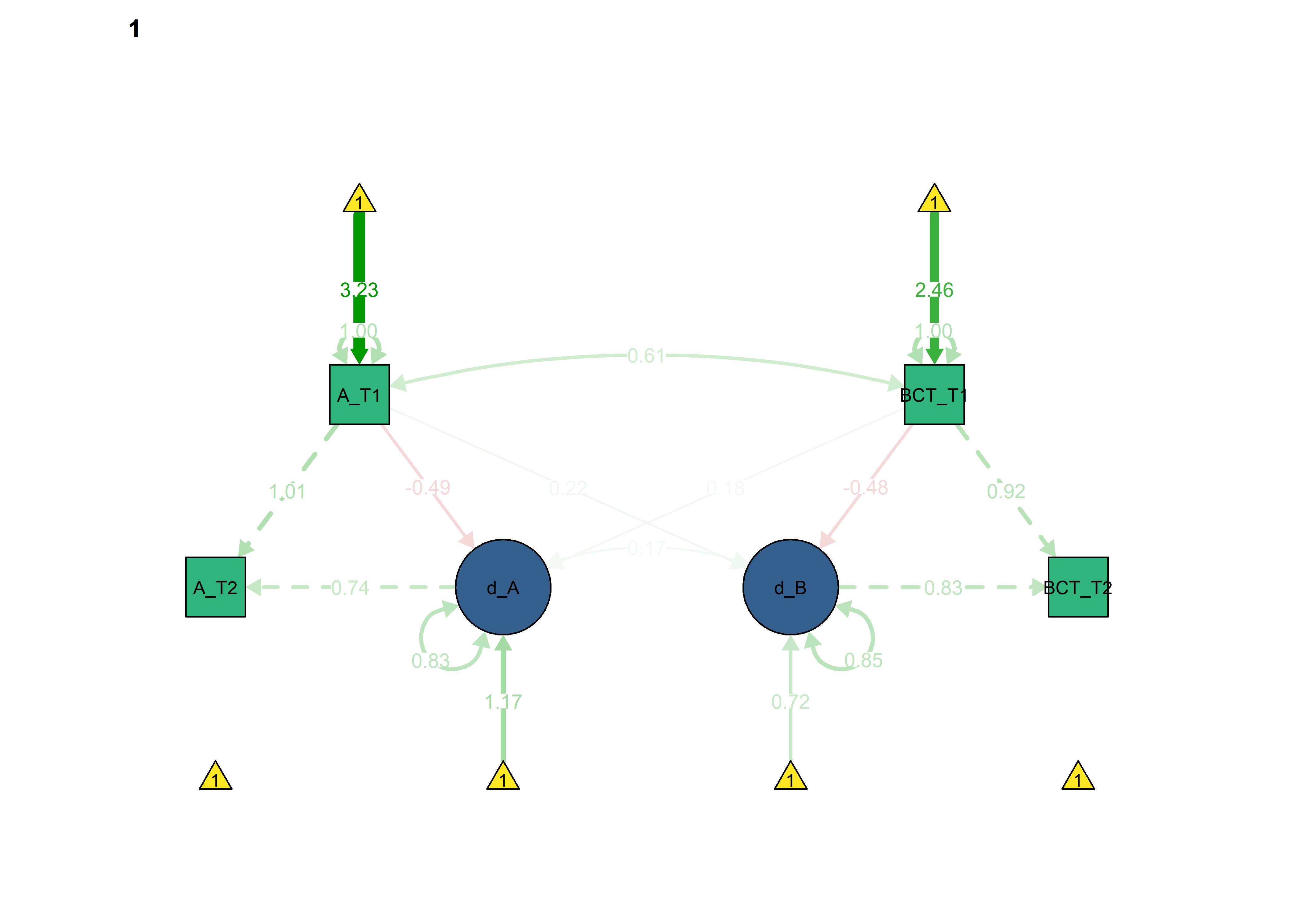
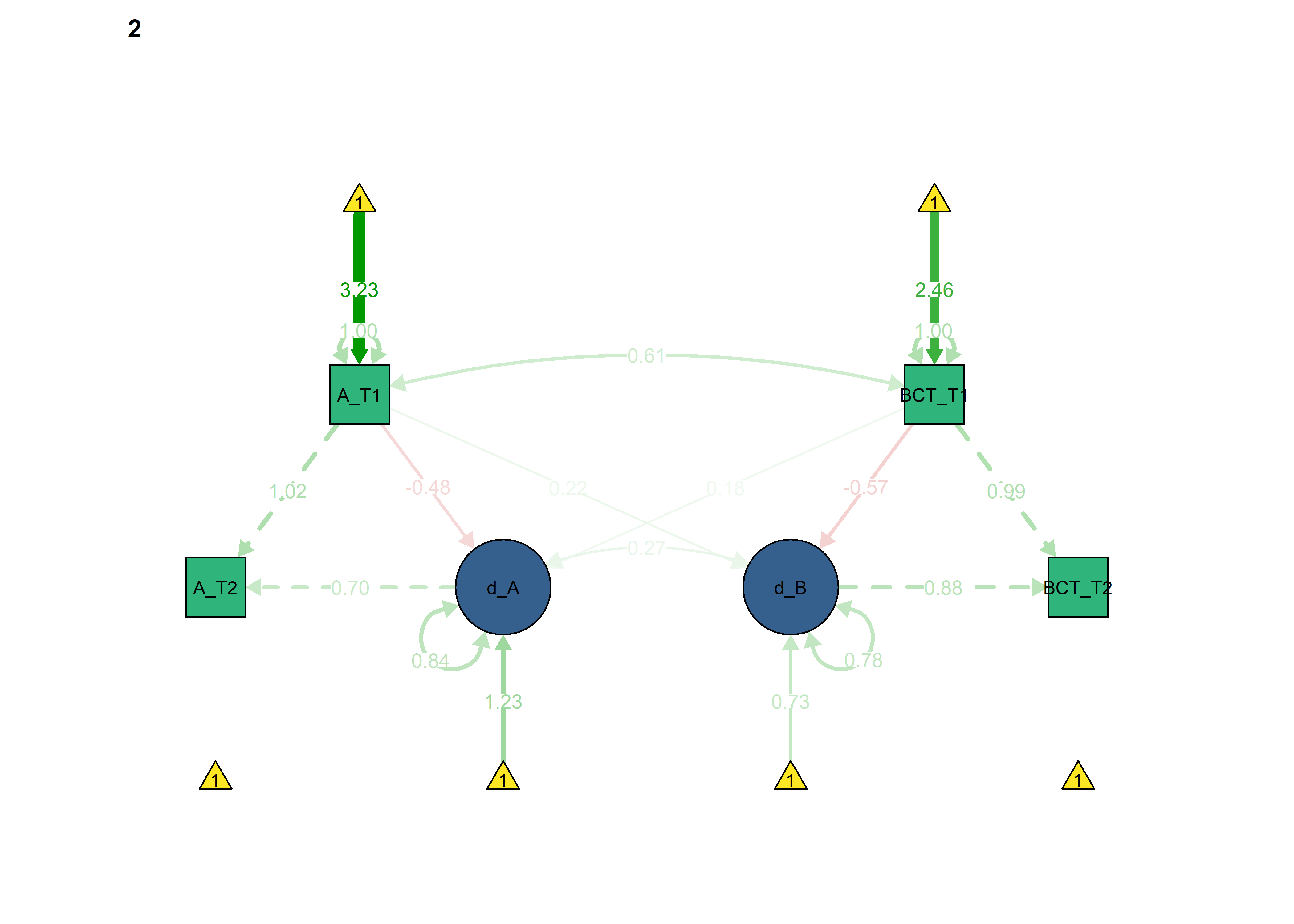
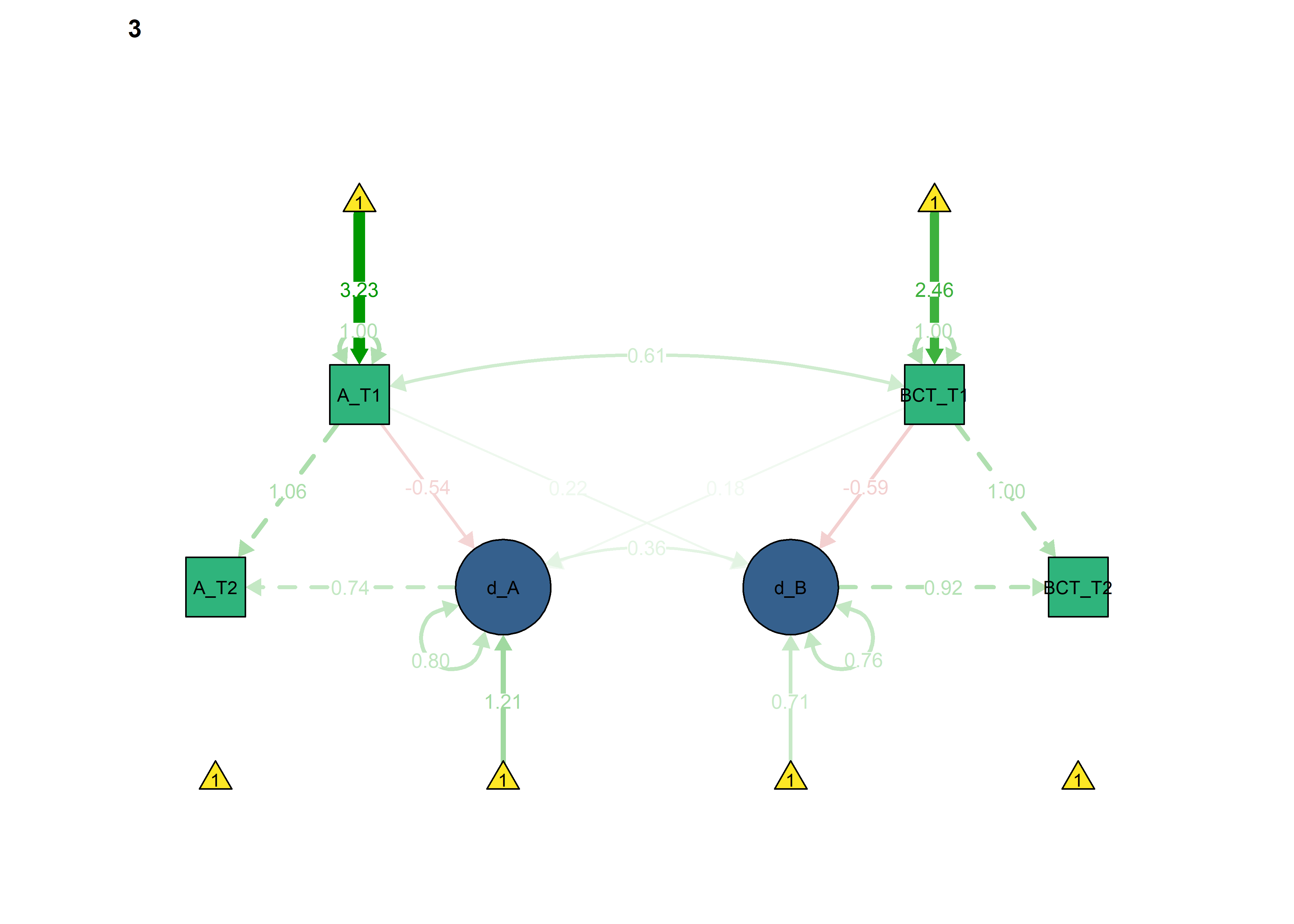
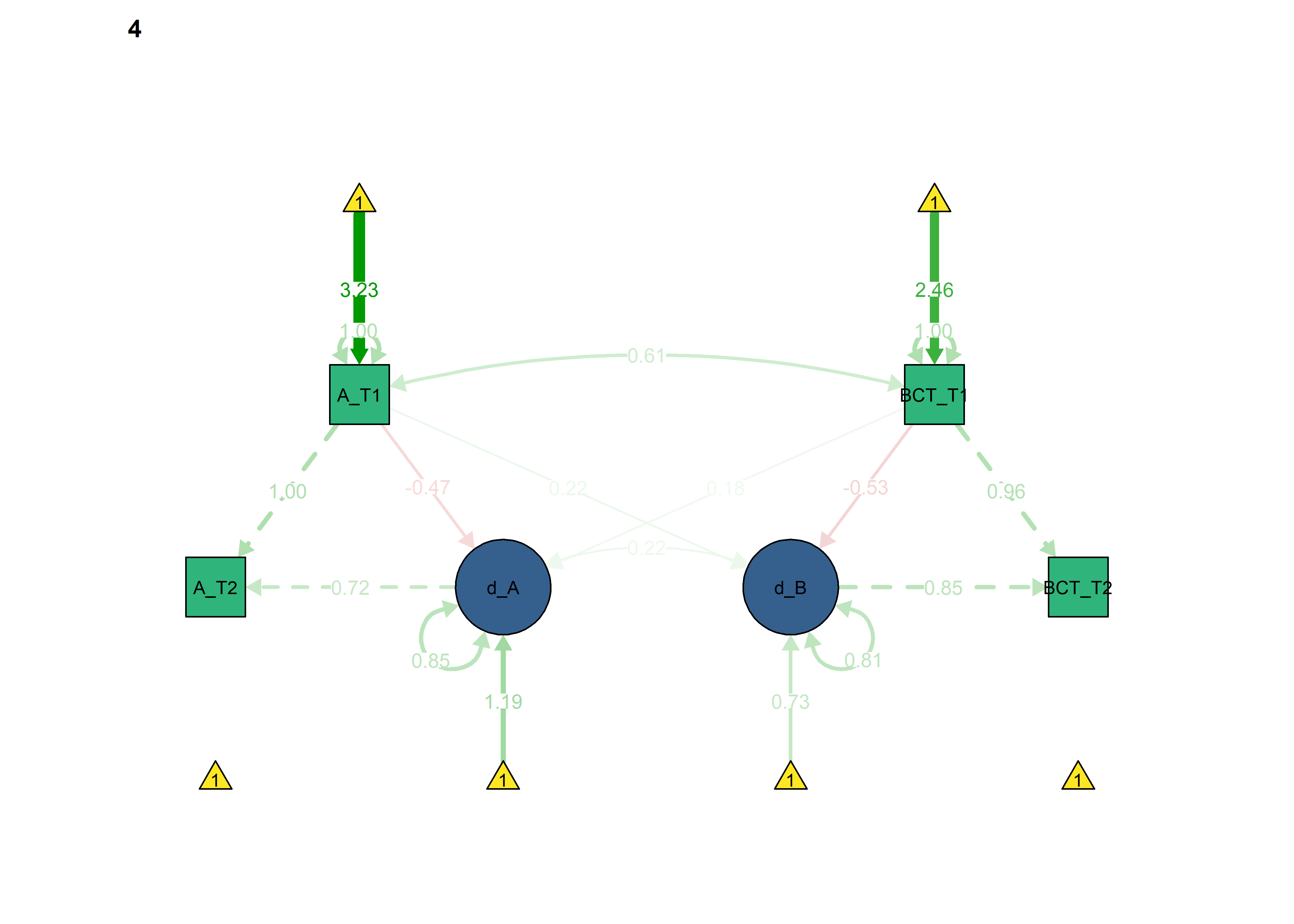
Constraints on basic model by group.equal
data_BLCS <- df %>% dplyr::select(
  track,
  Autonomous_T1 = PA_autonomous_T1,
  Autonomous_T2 = PA_autonomous_T3,
  frqbct_T1 = PA_frqbct_T1,
  frqbct_T2 = PA_frqbct_T3,
  agrbct_T1 = PA_agrbct_T1,
  agrbct_T2 = PA_agrbct_T3) %>%
  filter(track != "Other") %>%
  rowwise() %>%
  dplyr::mutate(BCTs_T1 = mean(c(frqbct_T1, agrbct_T1), na.rm = TRUE),
                BCTs_T2 = mean(c(frqbct_T2, agrbct_T2), na.rm = TRUE)) %>%
  dplyr::select(-contains("frq"), -contains("agr"))


#Fit the Bivariate Latent Change Score model to simulated data
BLCS_constrained2 <- '

Autonomous_T2 ~ 1 * Autonomous_T1     # This parameter regresses Autonomous_T2 perfectly on Autonomous_T1
d_Autonomous1 =~ 1 * Autonomous_T2    # This defines the latent change score factor as measured perfectly by scores on Autonomous_T2
d_Autonomous1 ~ 1                     # This estimates the intercept of the change score
Autonomous_T1 ~ 1  # This constrains the intercept of Autonomous_T1 to be identical across intervention and control groups
Autonomous_T2 ~ 0 * 1                 # This constrains the intercept of Autonomous_T2 to 0

BCTs_T2 ~ 1 * BCTs_T1     # This parameter regresses BCTs_T2 perfectly on BCTs_T1
d_BCTs1 =~ 1 * BCTs_T2    # This defines the latent change score factor as measured perfectly by scores on BCTs_T2
BCTs_T2 ~ 0 * 1           # This line constrains the intercept of BCTs_T2 to 0
BCTs_T2 ~~ 0 * BCTs_T2    # This fixes the variance of the BCTs_T1 to 0

d_Autonomous1 ~~  d_Autonomous1                     # This estimates the variance of the change scores
Autonomous_T1 ~~ Autonomous_T1  # This estimates the variance of the Autonomous_T1
Autonomous_T2 ~~ 0 * Autonomous_T2                  # This fixes the variance of the Autonomous_T2 to 0

d_BCTs1 ~ 1                            # This estimates the intercept of the change score
BCTs_T1 ~ 1        # This estimates the intercept of BCTs_T1
d_BCTs1 ~~ d_BCTs1                     # This estimates the variance of the change scores
BCTs_T1 ~~ BCTs_T1 # This estimates the variance of BCTs_T1

d_BCTs1 ~ Autonomous_T1 + BCTs_T1       # This estimates the autonomous to BCT coupling parameter and the BCT (T1) to BCT (T2) self-feedback
d_Autonomous1 ~ BCTs_T1 + Autonomous_T1 # This estimates the BCT to autonomous coupling parameter and the autonomous (T1) to autonomous (T2) self-feedback

Autonomous_T1 ~~ BCTs_T1                      # This estimates the Autonomous_T1 BCTs_T1 covariance
d_Autonomous1 ~~ d_BCTs1                      # This estimates the d_Autonomous and d_BCTs covariance
'

fitBLCS_constrained2 <- lavaan::lavaan(BLCS_constrained2,
                          data = data_BLCS,
                          estimator = 'mlr',
                          fixed.x = FALSE,
                          group = "track",
                          group.equal = c("intercepts", "means"),
                          missing = 'fiml')
## Warning in lav_data_full(data = data, group = group, cluster = cluster, : lavaan WARNING: some cases are empty and will be ignored:
##   79

lavaan::anova(fitBLCS, fitBLCS_constrained, fitBLCS_constrained2)
fitBLCS_constrained2 <- lavaan::lavaan(BLCS_constrained2,
                          data = data_BLCS,
                          estimator = 'mlr',
                          fixed.x = FALSE,
                          group = "track",
                          group.equal = c("intercepts"),
                          missing = 'fiml')
## Warning in lav_data_full(data = data, group = group, cluster = cluster, : lavaan WARNING: some cases are empty and will be ignored:
##   79

lavaan::anova(fitBLCS, fitBLCS_constrained, fitBLCS_constrained2)
lavaan::summary(fitBLCS_constrained2, fit.measures = TRUE, standardized = TRUE, rsquare = TRUE)
## lavaan (0.5-23.1097) converged normally after 90 iterations
##
## Used Total
## Number of observations per group
## BA 281 282
## HRC 213 213
## IT 163 163
## Nur 402 402
##
## Number of missing patterns per group
## BA 7
## HRC 4
## IT 3
## Nur 6
##
## Estimator ML Robust
## Minimum Function Test Statistic 59.080 57.004
## Degrees of freedom 6 6
## P-value (Chi-square) 0.000 0.000
## Scaling correction factor 1.036
## for the Yuan-Bentler correction
##
## Chi-square for each group:
##
## BA 16.400 15.824
## HRC 0.153 0.148
## IT 39.067 37.695
## Nur 3.460 3.338
##
## Model test baseline model:
##
## Minimum Function Test Statistic 1618.796 1066.992
## Degrees of freedom 24 24
## P-value 0.000 0.000
##
## User model versus baseline model:
##
## Comparative Fit Index (CFI) 0.967 0.951
## Tucker-Lewis Index (TLI) 0.867 0.804
##
## Robust Comparative Fit Index (CFI) 0.967
## Robust Tucker-Lewis Index (TLI) 0.866
##
## Loglikelihood and Information Criteria:
##
## Loglikelihood user model (H0) -4924.014 -4924.014
## Scaling correction factor 1.050
## for the MLR correction
## Loglikelihood unrestricted model (H1) -4894.474 -4894.474
## Scaling correction factor 1.161
## for the MLR correction
##
## Number of free parameters 50 50
## Akaike (AIC) 9948.028 9948.028
## Bayesian (BIC) 10196.282 10196.282
## Sample-size adjusted Bayesian (BIC) 10037.474 10037.474
##
## Root Mean Square Error of Approximation:
##
## RMSEA 0.183 0.179
## 90 Percent Confidence Interval 0.142 0.227 0.139 0.222
## P-value RMSEA <= 0.05 0.000 0.000
##
## Robust RMSEA 0.182
## 90 Percent Confidence Interval 0.141 0.227
##
## Standardized Root Mean Square Residual:
##
## SRMR 0.078 0.078
##
## Parameter Estimates:
##
## Information Observed
## Standard Errors Robust.huber.white
##
##
## Group 1 [BA]:
##
## Latent Variables:
## Estimate Std.Err z-value P(>|z|) Std.lv Std.all
## d_Autonomous1 =~
## Autonomous_T2 1.000 0.753 0.747
## d_BCTs1 =~
## BCTs_T2 1.000 1.051 0.869
##
## Regressions:
## Estimate Std.Err z-value P(>|z|) Std.lv Std.all
## Autonomous_T2 ~
## Autonomous_T1 1.000 1.000 0.990
## BCTs_T2 ~
## BCTs_T1 1.000 1.000 0.948
## d_BCTs1 ~
## Autonomous_T1 0.226 0.112 2.014 0.044 0.215 0.214
## BCTs_T1 -0.488 0.117 -4.168 0.000 -0.465 -0.533
## d_Autonomous1 ~
## BCTs_T1 0.056 0.079 0.707 0.479 0.074 0.085
## Autonomous_T1 -0.315 0.077 -4.099 0.000 -0.418 -0.417
##
## Covariances:
## Estimate Std.Err z-value P(>|z|) Std.lv Std.all
## Autonomous_T1 ~~
## BCTs_T1 0.725 0.071 10.206 0.000 0.725 0.634
## .d_Autonomous1 ~~
## .d_BCTs1 0.112 0.059 1.908 0.056 0.168 0.168
##
## Intercepts:
## Estimate Std.Err z-value P(>|z|) Std.lv Std.all
## .d_Atnm1 0.936 0.187 4.998 0.000 1.243 1.243
## Atnm_T1 (.p4.) 3.431 0.035 98.747 0.000 3.431 3.437
## .Atnm_T2 0.000 0.000 0.000
## .BCTs_T2 0.000 0.000 0.000
## .d_BCTs1 0.880 0.231 3.812 0.000 0.837 0.837
## BCTs_T1 (.14.) 2.833 0.037 75.766 0.000 2.833 2.472
##
## Variances:
## Estimate Std.Err z-value P(>|z|) Std.lv Std.all
## .BCTs_T2 0.000 0.000 0.000
## .d_Autonomous1 0.490 0.067 7.359 0.000 0.864 0.864
## Autonomous_T1 0.996 0.073 13.579 0.000 0.996 1.000
## .Autonomous_T2 0.000 0.000 0.000
## .d_BCTs1 0.900 0.095 9.500 0.000 0.815 0.815
## BCTs_T1 1.313 0.107 12.326 0.000 1.313 1.000
##
## R-Square:
## Estimate
## BCTs_T2 1.000
## d_Autonomous1 0.136
## Autonomous_T2 1.000
## d_BCTs1 0.185
##
##
## Group 2 [HRC]:
##
## Latent Variables:
## Estimate Std.Err z-value P(>|z|) Std.lv Std.all
## d_Autonomous1 =~
## Autonomous_T2 1.000 0.760 0.766
## d_BCTs1 =~
## BCTs_T2 1.000 0.972 0.804
##
## Regressions:
## Estimate Std.Err z-value P(>|z|) Std.lv Std.all
## Autonomous_T2 ~
## Autonomous_T1 1.000 1.000 1.070
## BCTs_T2 ~
## BCTs_T1 1.000 1.000 0.966
## d_BCTs1 ~
## Autonomous_T1 0.176 0.091 1.937 0.053 0.181 0.192
## BCTs_T1 -0.398 0.095 -4.184 0.000 -0.410 -0.478
## d_Autonomous1 ~
## BCTs_T1 0.134 0.058 2.304 0.021 0.177 0.206
## Autonomous_T1 -0.401 0.076 -5.251 0.000 -0.527 -0.559
##
## Covariances:
## Estimate Std.Err z-value P(>|z|) Std.lv Std.all
## Autonomous_T1 ~~
## BCTs_T1 0.677 0.090 7.524 0.000 0.677 0.547
## .d_Autonomous1 ~~
## .d_BCTs1 0.164 0.050 3.297 0.001 0.277 0.277
##
## Intercepts:
## Estimate Std.Err z-value P(>|z|) Std.lv Std.all
## .d_Atnm1 1.087 0.218 4.989 0.000 1.430 1.430
## Atnm_T1 (.p4.) 3.431 0.035 98.747 0.000 3.431 3.234
## .Atnm_T2 0.000 0.000 0.000
## .BCTs_T2 0.000 0.000 0.000
## .d_BCTs1 0.541 0.219 2.469 0.014 0.557 0.557
## BCTs_T1 (.14.) 2.833 0.037 75.766 0.000 2.833 2.427
##
## Variances:
## Estimate Std.Err z-value P(>|z|) Std.lv Std.all
## .BCTs_T2 0.000 0.000 0.000
## .d_Autonomous1 0.446 0.080 5.606 0.000 0.771 0.771
## Autonomous_T1 1.126 0.092 12.186 0.000 1.126 1.000
## .Autonomous_T2 0.000 0.000 0.000
## .d_BCTs1 0.788 0.097 8.094 0.000 0.835 0.835
## BCTs_T1 1.362 0.119 11.459 0.000 1.362 1.000
##
## R-Square:
## Estimate
## BCTs_T2 1.000
## d_Autonomous1 0.229
## Autonomous_T2 1.000
## d_BCTs1 0.165
##
##
## Group 3 [IT]:
##
## Latent Variables:
## Estimate Std.Err z-value P(>|z|) Std.lv Std.all
## d_Autonomous1 =~
## Autonomous_T2 1.000 0.683 0.567
## d_BCTs1 =~
## BCTs_T2 1.000 1.020 0.819
##
## Regressions:
## Estimate Std.Err z-value P(>|z|) Std.lv Std.all
## Autonomous_T2 ~
## Autonomous_T1 1.000 1.000 1.008
## BCTs_T2 ~
## BCTs_T1 1.000 1.000 0.964
## d_BCTs1 ~
## Autonomous_T1 0.335 0.096 3.479 0.001 0.328 0.398
## BCTs_T1 -0.581 0.104 -5.586 0.000 -0.569 -0.683
## d_Autonomous1 ~
## BCTs_T1 0.090 0.066 1.362 0.173 0.132 0.158
## Autonomous_T1 -0.234 0.074 -3.138 0.002 -0.342 -0.415
##
## Covariances:
## Estimate Std.Err z-value P(>|z|) Std.lv Std.all
## Autonomous_T1 ~~
## BCTs_T1 1.107 0.115 9.613 0.000 1.107 0.760
## .d_Autonomous1 ~~
## .d_BCTs1 0.201 0.061 3.304 0.001 0.343 0.343
##
## Intercepts:
## Estimate Std.Err z-value P(>|z|) Std.lv Std.all
## .d_Atnm1 0.508 0.150 3.380 0.001 0.745 0.745
## Atnm_T1 (.p4.) 3.431 0.035 98.747 0.000 3.431 2.825
## .Atnm_T2 0.000 0.000 0.000
## .BCTs_T2 0.000 0.000 0.000
## .d_BCTs1 0.453 0.193 2.347 0.019 0.444 0.444
## BCTs_T1 (.14.) 2.833 0.037 75.766 0.000 2.833 2.361
##
## Variances:
## Estimate Std.Err z-value P(>|z|) Std.lv Std.all
## .BCTs_T2 0.000 0.000 0.000
## .d_Autonomous1 0.421 0.060 7.058 0.000 0.902 0.902
## Autonomous_T1 1.474 0.135 10.889 0.000 1.474 1.000
## .Autonomous_T2 0.000 0.000 0.000
## .d_BCTs1 0.821 0.111 7.390 0.000 0.789 0.789
## BCTs_T1 1.440 0.121 11.895 0.000 1.440 1.000
##
## R-Square:
## Estimate
## BCTs_T2 1.000
## d_Autonomous1 0.098
## Autonomous_T2 1.000
## d_BCTs1 0.211
##
##
## Group 4 [Nur]:
##
## Latent Variables:
## Estimate Std.Err z-value P(>|z|) Std.lv Std.all
## d_Autonomous1 =~
## Autonomous_T2 1.000 0.768 0.765
## d_BCTs1 =~
## BCTs_T2 1.000 1.032 0.903
##
## Regressions:
## Estimate Std.Err z-value P(>|z|) Std.lv Std.all
## Autonomous_T2 ~
## Autonomous_T1 1.000 1.000 1.018
## BCTs_T2 ~
## BCTs_T1 1.000 1.000 0.970
## d_BCTs1 ~
## Autonomous_T1 0.190 0.064 2.973 0.003 0.184 0.188
## BCTs_T1 -0.500 0.061 -8.253 0.000 -0.485 -0.538
## d_Autonomous1 ~
## BCTs_T1 0.139 0.048 2.875 0.004 0.181 0.201
## Autonomous_T1 -0.385 0.056 -6.933 0.000 -0.502 -0.512
##
## Covariances:
## Estimate Std.Err z-value P(>|z|) Std.lv Std.all
## Autonomous_T1 ~~
## BCTs_T1 0.638 0.056 11.404 0.000 0.638 0.563
## .d_Autonomous1 ~~
## .d_BCTs1 0.139 0.040 3.483 0.000 0.218 0.218
##
## Intercepts:
## Estimate Std.Err z-value P(>|z|) Std.lv Std.all
## .d_Atnm1 1.022 0.145 7.038 0.000 1.331 1.331
## Atnm_T1 (.p4.) 3.431 0.035 98.747 0.000 3.431 3.358
## .Atnm_T2 0.000 0.000 0.000
## .BCTs_T2 0.000 0.000 0.000
## .d_BCTs1 0.928 0.171 5.428 0.000 0.899 0.899
## BCTs_T1 (.14.) 2.833 0.037 75.766 0.000 2.833 2.553
##
## Variances:
## Estimate Std.Err z-value P(>|z|) Std.lv Std.all
## .BCTs_T2 0.000 0.000 0.000
## .d_Autonomous1 0.479 0.047 10.093 0.000 0.813 0.813
## Autonomous_T1 1.044 0.060 17.419 0.000 1.044 1.000
## .Autonomous_T2 0.000 0.000 0.000
## .d_BCTs1 0.841 0.065 13.027 0.000 0.789 0.789
## BCTs_T1 1.231 0.075 16.386 0.000 1.231 1.000
##
## R-Square:
## Estimate
## BCTs_T2 1.000
## d_Autonomous1 0.187
## Autonomous_T2 1.000
## d_BCTs1 0.211
semPlot::semPaths(fitBLCS_constrained2,
what = "std",
ask = FALSE,
label.cex = .6,
label.scale = FALSE,
edge.label.cex = 0.75,
layout = "tree2",
intercepts = TRUE,
color = list(lat = viridis::viridis(3, begin = 0.3)[1],
man = viridis::viridis(3, begin = 0.3)[2],
int = viridis::viridis(3, begin = 0.3)[3]))